Understanding Asymptotic Notations: Big O, Big Omega, and Big Theta

The Essence of Asymptotic Analysis

In the previous lesson, we saw that an algorithm's complexity might be described by a function like $T(n)=n^2+n+3$. Asymptotic analysis is concerned with how this function behaves as the input size n becomes very large.

When n is large, the term with the highest growth rate (the highest-order term) dominates the function's value. In our example, $n^2$ grows much faster than n or the constant 3. For a large n, the other terms become insignificant in comparison. Asymptotic notation is a way to formalize this idea by ignoring lower-order terms and constant factors, allowing us to focus purely on the rate of growth.

Let's begin by exploring the three main notations used to describe these growth rates. We will be referring to an excellent article from Baeldung that provides clear, text-based explanations and formal definitions.

Big O Notation: The Upper Bound

In professional and interview settings, Big O is the most frequently discussed notation. It describes the upper bound on an algorithm's growth rate. It essentially answers the question: "In the worst-case scenario, how does the number of operations grow as the input size increases?"

Formally, we say a function $T(n)$ is in $O(g(n))$ (read as "Big O of g of n") if there exist positive constants c and $n_0$ such that:

Let's break this down:

• $T(n)$ is the actual complexity function of our algorithm.
• $g(n)$ represents a class of functions (like $n$, $n^2$, or $\log n$) that we use as a benchmark.
• The inequality tells us that, for some constant c, our function $T(n)$ will never grow faster than $c\cdot g(n)$ once the input n is large enough (i.e., greater than $n_0$).

To get a deeper understanding, please read the following sections from the Baeldung article.

As the article explains, while a function like $T(n)=n^2+n+3$ is technically $O(n^3)$ and $O(2^n)$, those are "loose" upper bounds. We always aim to provide the tightest possible upper bound, which in this case is $O(n^2)$. When you hear someone state an algorithm's Big O complexity, they are almost always referring to this tightest upper bound.

Big Omega (Ω) Notation: The Lower Bound

While Big O tells us the worst-case growth, Big Omega (Ω) tells us about the lower bound. It answers the question: "What is the best-case growth rate for this algorithm?"

Formally, a function $T(n)$ is in $\Omega (g(n))$ if there exist positive constants c and $n_0$ such that:

Notice the only change from the Big O definition is the direction of the inequality. $T(n)$ is guaranteed to grow at least as fast as $c\cdot g(n)$.

Let's continue with the same Baeldung article to see how this works.

For the function $T(n)=n^2+n+3$, we can say it is $\Omega (n^2)$ because $n^2+n+3\ge 1\cdot n^2$ for all positive n. Just like with Big O, we seek the tightest bound. While it's also $\Omega (n)$ and $\Omega (\log n)$, the most informative statement is that its growth is at least quadratic, i.e., $\Omega (n^2)$.

Big Theta (Θ) Notation: The Tight Bound

When an algorithm's growth is bounded both from above and below by the same class of function, we use Big Theta (Θ) notation. This is the most precise description of an algorithm's complexity, indicating an exact bound.

Formally, a function $T(n)$ is in $\Theta (g(n))$ if there exist positive constants $c_1$, $c_2$, and $n_0$ such that:

Essentially, $T(n)$ is $\Theta (g(n))$ if and only if it is both $O(g(n))$ and $\Omega (g(n))$. The function's growth is "sandwiched" between two scaled versions of $g(n)$.

Let's read the final piece of the Baeldung article.

Since our example function $T(n)=n^2+n+3$ is both $O(n^2)$ and $\Omega (n^2)$, we can say it is $\Theta (n^2)$. This tells us its growth is exactly quadratic.

A Visual Summary and a Key Distinction

The following image provides a great visual summary of the three notations.

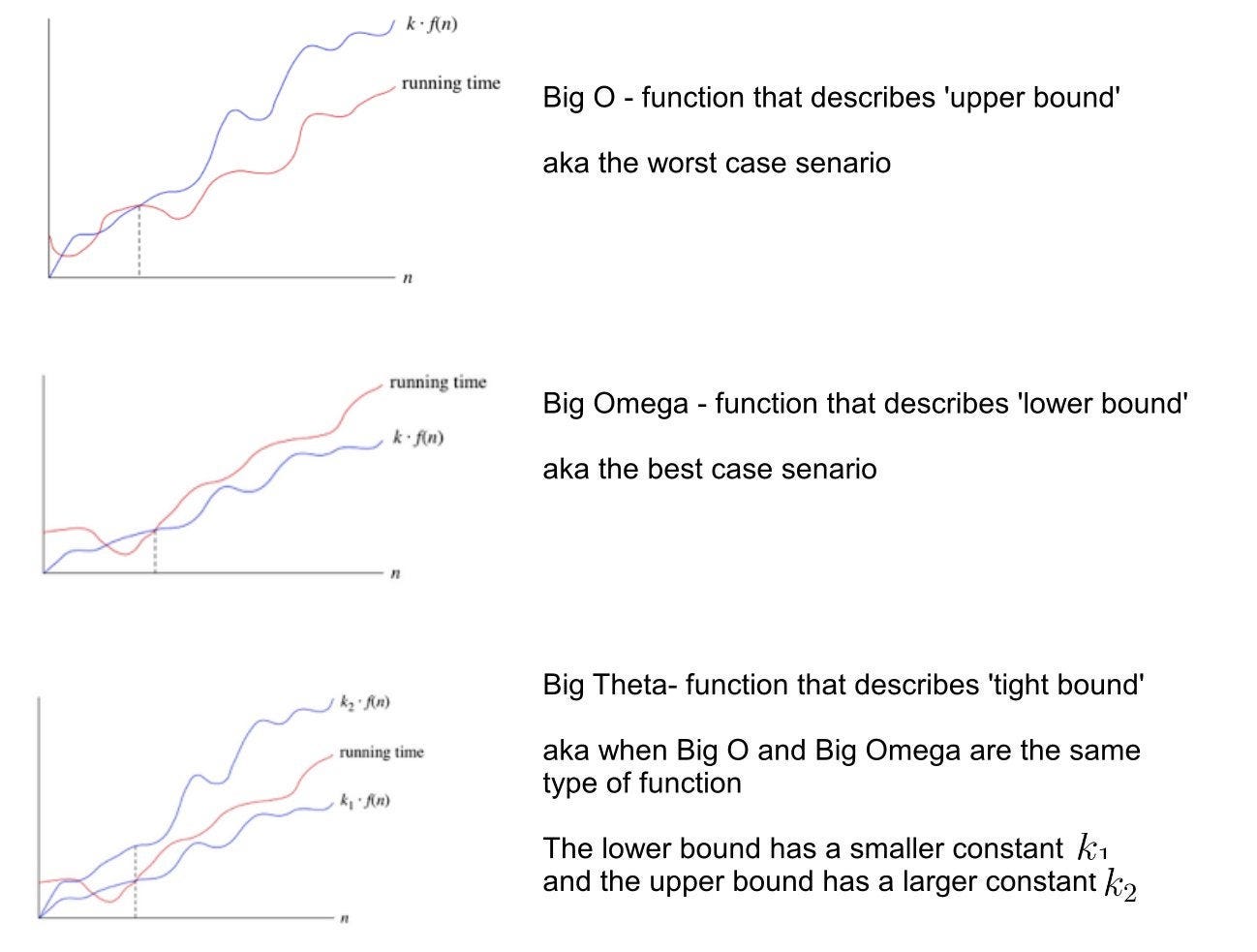
A common point of confusion is mixing up asymptotic notations with an algorithm's best, average, and worst-case scenarios. It's a subtle but critical distinction:

• Best/Worst/Average Case refers to different scenarios based on the input, each resulting in a specific complexity function. For example, Insertion Sort's best-case input is a sorted array, while its worst-case is a reverse-sorted array.
• Big O/Omega/Theta are notations used to describe the growth of any function, including the functions that arise from best-case or worst-case analysis.

For instance, the worst-case time complexity of Insertion Sort is described by a quadratic function, let's say $T_{worst}(n)=a{n}^2+bn+c$. We can then say that this worst-case complexity is $\Theta (n^2)$. We could also make weaker statements, like it's $O(n^2)$ or $\Omega (n)$, but the tightest description is $\Theta (n^2)$.

To solidify these differences, please read the clear definitions from the FAQ section of this "Built In" article.

Conclusion

In this lesson, we have equipped ourselves with the precise mathematical language to describe algorithmic efficiency. Let's recap the key distinctions:

• Big O (O) describes an upper bound on the growth rate. It is often used to characterize the worst-case performance of an algorithm.
• Big Omega (Ω) describes a lower bound. It's useful for defining the best-case performance.
• Big Theta (Θ) describes a tight bound. It provides the most precise classification when an algorithm's growth is bounded both above and below by the same function family.

In practice, you will find that Big O is the most common notation used. When a developer says an algorithm is "Big O of n-squared," they are typically communicating the tightest upper bound, which implies that the worst-case performance grows quadratically.

Now that we have the theoretical tools for describing complexity, our next lesson will focus on applying them. We will analyze simple iterative code structures, such as single and nested loops, to determine their time complexity using the notations you've learned today.