Calculus-Based Projectile Motion on Inclined Planes with Air Resistance

1. Projectile Motion on an Inclined Plane

Standard projectile motion formulas assume a horizontal ground, meaning the acceleration vector $\vec{g}$ is always perpendicular to the horizontal displacement. On an inclined plane, this is no longer true. The "ground" is tilted, and simply applying the old formulas will lead to incorrect results.

The most effective strategy is to redefine our frame of reference. Instead of a horizontal x-axis and vertical y-axis, we align our coordinate system with the incline itself.

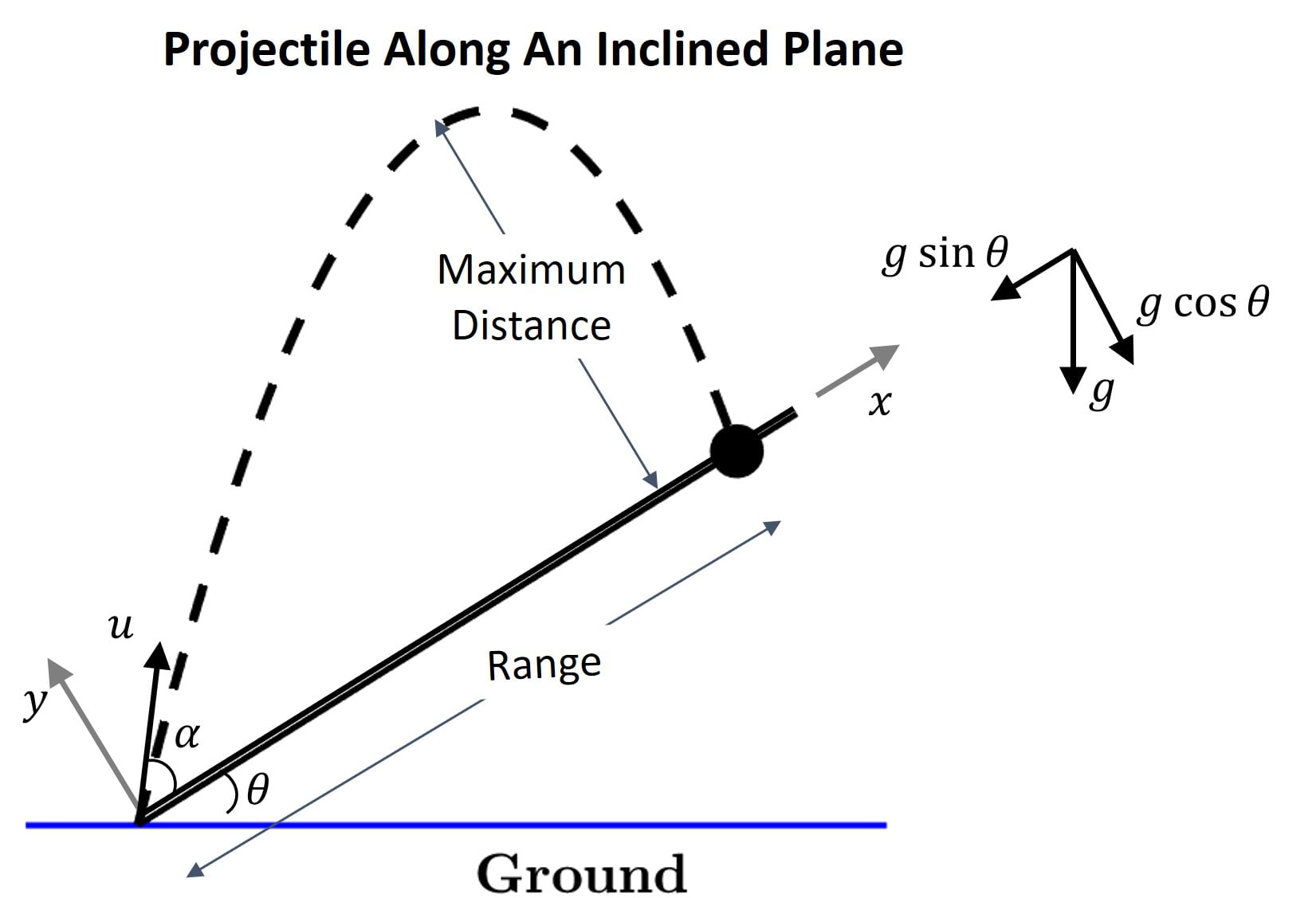
With this rotated coordinate system, the motion is governed by constant accelerations, just not the ones you're used to:

• Along the x-axis (parallel to the incline): $a_x=-g\sin \theta$
• Along the y-axis (perpendicular to the incline): $a_y=-g\cos \theta$

Once you have these components, you can treat the motion along each axis independently, just as you would in a standard projectile problem. The initial velocity $\vec{u}$ must also be resolved into components $u_x$ and $u_y$ along these new axes.

The following video provides a clear walkthrough of this technique to derive the time of flight and range along the incline.

The key formulas derived from this method are:

• Time of Flight (T): Found by analyzing the 'y' motion. The total displacement in the y-direction is zero. Using $s_y=u_{y}t+\frac{1}{2}{a}_y{t}^2$, we get: $$T=\frac{2u_y}{|a_y|}=\frac{2u\sin \alpha }{g\cos \theta }$$ where $\theta$ is the angle of the incline and $\alpha$ is the angle of projection relative to the incline.
• Range (R): Found by using the time of flight $T$ in the 'x' motion equation, $s_x=u_{x}T+\frac{1}{2}{a}_x{T}^2$. $$R=(u\cos \alpha )T+\frac{1}{2}(-g\sin \theta )T^2$$

JEE Advanced problems often test special conditions, such as:

• Finding the angle of projection for maximum range on the incline.
• Conditions where the projectile strikes the incline perpendicularly or horizontally.

These require you to apply the kinematic equations and then use calculus or vector conditions to solve for the specific constraint. For instance, to strike perpendicularly, the final velocity component along the incline ($v_x$) must be zero.

Let's see this technique applied to a quintessential JEE Advanced problem involving two inclined planes. The choice of coordinate system is paramount here.

To solidify your grasp on the variety of problems related to inclined planes, you can explore the following resource. It contains problems on maximum range, perpendicular collisions, and other common variations.

2. Projectile Motion with Air Resistance

We now turn to a case where the acceleration is no longer constant. Air resistance, or drag, is a force that opposes motion and typically depends on the velocity of the object. This velocity dependence means Newton's second law becomes a differential equation.

The drag force $F_d$ is often modeled in two ways:

1. Linear Drag: $F_d\propto v$. Analytically solvable and a good introduction to the method.
2. Quadratic Drag: $F_d\propto v^2$. More realistic for many macroscopic objects but often leads to more complex integrals.

For both models, the core strategy is the same:

1. Write Newton's second law in vector or component form: $m\vec{a}=m\vec{g}+{\vec{F}}_d$.
2. Since $\vec{a}=\frac{d\vec{v}}{dt}$ and $\vec{v}=\frac{d\vec{r}}{dt}$, this gives you a system of differential equations.
3. Solve these equations by integration, using the initial conditions (initial position and velocity).

Linear Drag Model (${\vec{F}}_d=-k\vec{v}$)

Let's analyze the solvable case of linear drag. The following resource provides a complete, calculus-based derivation.

Quadratic Drag Model and the $v\frac{dv}{ds}$ Technique

For the more realistic quadratic drag model ($F_d=k{v}^2$), solving for motion as a function of time can be very difficult. For problems asking for velocity as a function of position (e.g., "find the speed when it hits the ground"), a powerful technique is to change the variable of integration from time $t$ to displacement $s$. We use the chain rule to write acceleration as:

This transforms Newton's law $F=ma$ into $F=mv\frac{dv}{ds}$, which can be rearranged and integrated:

The following Physics Galaxy video demonstrates this exact technique for a vertical throw problem with quadratic air drag, a classic advanced problem.

This method of relating velocity to position is extremely useful for any problem where force is a function of velocity or position, and it will be a recurring theme in our study of mechanics.

Conclusion

Today we tackled two significant extensions of projectile motion that are representative of the challenges posed in the JEE Advanced exam. You have learned how to move beyond simple formulas and apply fundamental principles with calculus.

Key Takeaways:

• Projectile on an Incline: The most effective method is to rotate the coordinate system to align with the incline. Resolve the initial velocity and gravitational acceleration into components in this new system and apply constant acceleration kinematics.
• Projectile with Air Resistance: This is a variable acceleration problem that must be solved using differential equations.
  • Set up Newton's second law: $m\vec{a}=\sum \vec{F}$.
  • Substitute $\vec{a}=d\vec{v}/dt$ and integrate to find velocity and position as functions of time.
  • For problems where force is a function of velocity and you need to relate velocity to position, use the powerful substitution $a=v\frac{dv}{ds}$.

In our next lesson, we will continue our exploration of variable acceleration by examining problems where the force is a function of position, such as in systems with non-linear springs. This will further solidify your mastery of solving equations of motion through integration.