Second Quantization of Two-Particle Operators

Hello! In our last lesson, we developed a powerful tool for expressing single-particle operators like kinetic energy in the language of second quantization. We saw that an operator $O^$ can be written as $\sum_{α, β} ⟨ α ∣ o^∣ β ⟩ c_{α}^{†} c_{β}$ , which we interpreted as a sum over all possible single-particle transitions weighted by their quantum amplitudes.

This lesson addresses the heart of many-body physics: interactions. We will extend our formalism to handle two-particle operators, which describe forces between particles, with the Coulomb interaction being the most important example. By the end of this lesson, you will be able to write any two-particle interaction in second-quantized form. This is the final fundamental tool we need before we can begin constructing and analyzing the Hubbard model itself.

The General Rule for Two-Particle Operators

In first quantization, a two-particle operator is typically a sum over all distinct pairs of particles:

V^= \frac{1}{2} i \neq = j \sum v (r_{i}, r_{j})

The factor of $1/2$ corrects for double-counting each pair. Just as with single-particle operators, dealing with this form while respecting fermionic antisymmetry is extremely cumbersome for large $N$ .

The second-quantized representation provides a compact and elegant solution. The general "dictionary" for translating any two-particle operator into second quantization is:

V^= \frac{1}{2} α, β, γ, δ \sum ⟨ α, β ∣ v ∣ γ, δ ⟩ c_{α}^{†} c_{β}^{†} c_{δ} c_{γ}

Let's unpack this important expression.

The Matrix Element: The coefficient $⟨ α, β ∣ v ∣ γ, δ ⟩$ is the two-particle matrix element. It's calculated by integrating the interaction potential against the wavefunctions of the initial and final states:
$⟨ α, β ∣ v ∣ γ, δ ⟩ = \iint d^{3} r_{1} d^{3} r_{2} ϕ_{α}^{*} (r_{1}) ϕ_{β}^{*} (r_{2}) v (r_{1}, r_{2}) ϕ_{γ} (r_{1}) ϕ_{δ} (r_{2})$
This integral represents the amplitude for a process where a particle in state $γ$ at position $r_{1}$ and a particle in state $δ$ at position $r_{2}$ interact and scatter into states $α$ (at $r_{1}$ ) and $β$ (at $r_{2}$ ).
The Operator String: The sequence of operators $c_{α}^{†} c_{β}^{†} c_{δ} c_{γ}$ provides the physical mechanism. It annihilates a particle in state $γ$ , annihilates another in state $δ$ , then creates one in state $β$ , and finally creates one in state $α$ . This four-operator string is the hallmark of a two-body interaction in second quantization. It describes a scattering event where two particles are destroyed and two new ones are created.

The following video provides a helpful conceptual picture for this scattering process.

4- Operators in Second Quantization - Course on Quantum Many-Body Physics

This video from the "Course on Quantum Many-Body Physics" by Luis Gregorio Dias offers a simple pictorial way to think about one- and two-body operators.

Watch the short segment from this point. The video visualizes a single-particle operator as scattering a particle from one state to another, and a two-particle operator as a more complex event where two incoming particles interact and scatter into two outgoing states. This diagrammatic thinking is a precursor to more formal methods like Feynman diagrams.

A Crucial Note on Operator Ordering

For fermions, the order of operators is critical. Notice the annihilation operators are written as $c_{δ} c_{γ}$ . The standard convention for the matrix element $⟨ α, β ∣ v ∣ γ, δ ⟩$ maps indices as $(α, β) \leftarrow (γ, δ)$ , but the operators act in the "reverse" order $c_{δ} c_{γ}$ . Swapping them to $c_{γ} c_{δ}$ would introduce a minus sign due to the anticommutation relations, which could incorrectly flip the sign of your interaction. This is a frequent source of error, so it's worth committing to memory.

The following reading formally presents this rule and its derivation.

1 Quantum mechanics for one particle - review of notation

These lecture notes by Mona Berciu formally state the theorem for two-particle operators and provide a detailed example for the Coulomb interaction.

First, read the statement of the theorem for two-particle operators. You can find it in the section starting with "Theorem: If ˆB..." (p. 8). Pay close attention to Eq. (10) and the capitalized note immediately following it, which emphasizes the critical importance of the operator ordering. Next, follow the detailed derivation for a spin-independent two-particle interaction in the momentum basis (p. 10). This section applies the general theorem to derive Eq. (13), the second-quantized form of the Coulomb interaction. Focus on how the Fourier transform of the potential naturally leads to momentum conservation.

Example 1: Coulomb Interaction in Momentum Space

As shown in the reading from Berciu's notes, applying the general formula to a translationally invariant system in a plane-wave basis ( $∣ k, σ ⟩$ ) gives a very intuitive result. The interaction Hamiltonian becomes:

V^= \frac{1}{2 V} k, k^{'} σ, σ^{'} \sum q \sum v (q) c_{k - q, σ}^{†} c_{k^{'} + q, σ^{'}}^{†} c_{k^{'}, σ^{'}} c_{k, σ}

Here, $v (q)$ is the Fourier transform of the interaction potential $v (r)$ .

This expression beautifully captures the physics of a two-body collision. A particle in state $(k, σ)$ and another in state $(k^{'}, σ^{'})$ interact. They exchange momentum $q$ , and scatter into new final states $(k - q, σ)$ and $(k^{'} + q, σ^{'})$ . The total momentum $(k - q) + (k^{'} + q) = k + k^{'}$ is conserved, as expected for an interaction that only depends on the relative distance between particles. The spin of each particle is also conserved because the Coulomb interaction is spin-independent.

Example 2: The On-Site Hubbard Interaction

Now, let's turn to the most important example for this course. Instead of delocalized plane waves, consider electrons in orbitals tightly bound to specific atoms on a crystal lattice. We use a basis of Wannier states, $∣ i, σ ⟩$ , where $i$ labels the lattice site and $σ$ is the spin.

The full Coulomb interaction between all electrons on all sites is still immensely complicated. The crucial simplification that leads to the Hubbard model is to assume that the interaction is only significant when two electrons are on the exact same site. All inter-site interactions are ignored. This is a reasonable approximation for materials where electrons are strongly localized and screening effects are strong.

Under this "on-site" approximation, the only non-zero matrix elements in the two-body operator are those where all four state indices refer to the same site: $i = j = k = l$ . The interaction strength is then given by a single parameter, $U$ :

U = ⟨ i, i ∣ v ∣ i, i ⟩ = \iint d^{3} r_{1} d^{3} r_{2} ∣ ϕ_{i} (r_{1}) ∣^{2} v (r_{1}, r_{2}) ∣ ϕ_{i} (r_{2}) ∣^{2}

This $U$ represents the energy cost of putting two electrons on the same atomic orbital.

Plugging this into the general two-particle operator formula gives:

V^_{on-site} = \frac{1}{2} i, σ, σ^{'} \sum U c_{iσ}^{†} c_{i σ^{'}}^{†} c_{i σ^{'}} c_{iσ}

Since fermions cannot occupy the same state, the Pauli principle dictates that this term is only non-zero if the two electrons have opposite spins, $σ \neq = σ^{'}$ . For a spin-1/2 system, this means we must have one spin-up and one spin-down electron. The sum reduces to:

V^_{on-site} = U i \sum c_{i ↑}^{†} c_{i ↓}^{†} c_{i ↓} c_{i ↑}

(The factor of $1/2$ disappears because the sum over $σ \neq = σ^{'}$ gives two identical terms: $(↑, ↓)$ and $(↓, ↑)$ ).

This expression can be simplified even further. Because operators for different spins commute, and the number operator $n^_{i ↓} = c_{i ↓}^{†} c_{i ↓}$ is a bilinear, it commutes with the spin-up operators. We can therefore rearrange the terms:

c_{i ↑}^{†} c_{i ↓}^{†} c_{i ↓} c_{i ↑} = c_{i ↑}^{†} (n^_{i ↓}) c_{i ↑} = n^_{i ↓} c_{i ↑}^{†} c_{i ↑} = n^_{i ↑} n^_{i ↓}

So, the final, remarkably simple form for the on-site interaction is:

H^_{U} = U i \sum n^_{i ↑} n^_{i ↓}

This is the celebrated Hubbard $U$ term. It adds an energy penalty $U$ to the system for every site $i$ that is "doubly occupied" (i.e., has one spin-up and one spin-down electron). This simple term is responsible for a vast range of fascinating phenomena in correlated electron systems, including the metal-insulator transition.

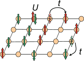
This image illustrates the two key processes in the Hubbard model. The term we just derived, the on-site repulsion U, penalizes the double occupancy of a lattice site. The hopping term, t, which we will combine with U in the next module, describes the kinetic energy of electrons moving between adjacent sites.

Conclusion

We have now completed our foundational toolkit for many-body physics. We have moved from the cumbersome machinery of first quantization to the powerful and elegant language of creation and annihilation operators.

Today's key takeaways are:

A two-particle operator is represented in second quantization by a sum over four-operator strings: $V^= \frac{1}{2} \sum_{α, β, γ, δ} ⟨ α, β ∣ v ∣ γ, δ ⟩ c_{α}^{†} c_{β}^{†} c_{δ} c_{γ}$ .
This operator string describes a scattering process where particles in states $γ$ and $δ$ are annihilated, and particles in states $α$ and $β$ are created.
The specific ordering of annihilation operators, $c_{δ} c_{γ}$ , is crucial for fermions and must be respected.
In momentum space, the Coulomb interaction describes the exchange of momentum between scattering particles.
In a real-space basis of localized orbitals, making the on-site approximation reduces the Coulomb interaction to the simple and intuitive Hubbard $U$ term: $U \sum_{i} n^_{i ↑} n^_{i ↓}$ .

We have now defined states and operators in this new language. In our next lesson, we will cover our final topic in this module: how these operators transform when we change from one single-particle basis to another, for instance, from real space to momentum space. This will be essential for diagonalizing Hamiltonians and finding their energy spectra.

Recommended resources

The General Rule for Two-Particle Operators

A Crucial Note on Operator Ordering

Example 1: Coulomb Interaction in Momentum Space

Example 2: The On-Site Hubbard Interaction

Conclusion