Basis Transformations for Creation/Annihilation Operators

Welcome to the final lesson in our module on the foundations of second quantization. In the previous lessons, you learned how to represent states, single-particle operators, and two-particle interaction operators using the formalism of creation and annihilation operators. We concluded by deriving the Hubbard $U$ term, $U \sum_{i} n^_{i ↑} n^_{i ↓}$ , which describes on-site electron repulsion in a real-space lattice basis.

While expressing a Hamiltonian in a particular basis is a crucial first step, it is often not the most convenient basis for solving the problem. For systems with translational symmetry, like a crystal lattice, the problem often simplifies dramatically when transformed into a basis of definite momentum. This is deeply analogous to solving a system of coupled classical oscillators by transforming to normal modes, where each mode oscillates independently.

In this lesson, you will learn the general procedure for changing the basis of creation and annihilation operators. We will then apply this technique to the essential transformation between the real-space (site) basis and the momentum-space basis. This skill is the final piece of our foundational toolkit and will be immediately applied in the next module to solve the tight-binding model.

The Power of the Right Basis: An Analogy

Before diving into the quantum formalism, let's revisit a concept from classical mechanics. A system of coupled oscillators, described in terms of the positions of individual masses, has a complicated Hamiltonian where the motion of one mass is linked to its neighbors. However, by performing a Fourier transform, we can describe the system in terms of independent normal modes, each with its own frequency. The Hamiltonian becomes a simple sum over these uncoupled modes.

The video below gives an excellent overview of this exact idea. While it deals with a classical system, the mathematical strategy and the physical intuition are identical to what we are about to do for quantum particles on a lattice.

Full Explanation of Second Quantization | Advanced Quantum Mechanics

This video from Bari Science Lab provides a full derivation of how a Fourier transform diagonalizes the Hamiltonian for a classical chain of coupled oscillators.

First, watch the introduction here to grasp the core concept of decoupling oscillators by moving to momentum space. Next, watch the detailed transformation of the kinetic energy term from position space to momentum space. Finally, see how the more complex potential energy (coupling) term is also diagonalized in the segment from here. Focus on the overall strategy: starting with a coupled real-space Hamiltonian and ending with a decoupled momentum-space Hamiltonian. The algebraic details are less important than understanding why this transformation is so powerful.

General Transformation of Operators

Now, let's formalize this for our second-quantized operators. Suppose we have two different complete, orthonormal single-particle bases, ${∣ α ⟩}$ and ${∣ β ⟩}$ . We can define a set of fermionic creation and annihilation operators for each basis, let's say $c_{α}^{†}, c_{α}$ and $d_{β}^{†}, d_{β}$ . How do we relate them?

The key is the completeness relation, or the resolution of the identity, which allows us to express any state from one basis as a linear combination of states in the other.

∣ β ⟩ = α \sum ∣ α ⟩ ⟨ α ∣ β ⟩

The coefficients of this expansion, $⟨ α ∣ β ⟩$ , are the overlaps between the basis states.

By definition, the creation operators generate these states from the vacuum: $d_{β}^{†} ∣0 ⟩ = ∣ β ⟩$ and $c_{α}^{†} ∣0 ⟩ = ∣ α ⟩$ . Substituting these into the expansion above gives:

d_{β}^{†} ∣0 ⟩ = α \sum ⟨ α ∣ β ⟩ (c_{α}^{†} ∣0 ⟩) = (α \sum ⟨ α ∣ β ⟩ c_{α}^{†}) ∣0 ⟩

Since this must hold true, we can equate the operators themselves. This gives us the fundamental transformation law for creation operators:

d_{β}^{†} = α \sum ⟨ α ∣ β ⟩ c_{α}^{†}

To find the rule for annihilation operators, we simply take the Hermitian conjugate of this equation:

d_{β} = (d_{β}^{†})^{†} = (α \sum ⟨ α ∣ β ⟩ c_{α}^{†})^{†} = α \sum ⟨ α ∣ β ⟩^{*} c_{α} = α \sum ⟨ β ∣ α ⟩ c_{α}

So, a "new" operator is just a linear combination of the "old" operators, weighted by the overlaps between the new and old basis states.

The following short video provides a very clear step-by-step derivation of these rules and verifies that the transformation correctly preserves the anticommutation relations.

Changing basis in second quantization

The video "Changing basis in second quantization" by Professor M does Science walks through the derivation we just outlined.

Watch the video from the beginning until this point. Pay close attention to how the resolution of the identity is used to derive the transformation rules for creation and annihilation operators, and how the original anticommutation relations are used to prove that the new operators also obey them.

For a written summary of this fundamental rule, you can refer to the following text.

Chapter 2 Second Quantisation

These lecture notes from the University of Cambridge provide a concise, formal statement of the basis change transformation law.

In the section "Notations and Definitions", find the subsection titled "Change of basis". Focus on Eq. (2.3), which presents the same transformation rules we derived above.

Application: From Real Space to Momentum Space

Let's now apply this machinery to the most common basis change in condensed matter physics: transforming from localized atomic orbitals on a lattice to delocalized plane waves with definite momentum.

Real-space basis: The states are $∣ j, σ ⟩$ , representing an electron with spin $σ$ localized at lattice site $j$ . The corresponding operators are $c_{j σ}^{†}$ and $c_{j σ}$ .
Momentum-space basis: The states are $∣ k, σ ⟩$ , representing an electron with spin $σ$ in a Bloch state with crystal momentum $k$ . The corresponding operators are $c_{k σ}^{†}$ and $c_{k σ}$ .

For a one-dimensional lattice with $N$ sites, periodic boundary conditions, and a lattice constant $a$ , the overlap between these basis states is given by the discrete Fourier transform relationship:

⟨ j ∣ k ⟩ = \frac{1}{N} e^{ik r_{j}}

where $r_{j} = j a$ is the position of the $j$ -th site.

Using our general transformation rules, we can immediately write down the relationship between the operators:

c_{k σ}^{†} = j = 1 \sum N ⟨ j ∣ k ⟩ c_{j σ}^{†} = \frac{1}{N} j \sum e^{ik r_{j}} c_{j σ}^{†}

The inverse transformation is found by using the overlap $⟨ k ∣ j ⟩ = ⟨ j ∣ k ⟩^{*} = \frac{1}{N} e^{- ik r_{j}}$ :

c_{j σ}^{†} = k \sum ⟨ k ∣ j ⟩ c_{k σ}^{†} = \frac{1}{N} k \sum e^{- ik r_{j}} c_{k σ}^{†}

Here, the sum over $k$ is over the $N$ allowed discrete momentum values in the first Brillouin zone.

The following reading provides a detailed walkthrough of this transformation and uses it to diagonalize the non-interacting part of the Hubbard model.

Elementary Introduction to the Hubbard Model

This document by Richard Scalettar provides a clear introduction to the Hubbard model and its solution in the non-interacting limit, which relies on the basis change we are studying.

Begin reading the section titled "LIMIT OF NO INTERACTIONS" (p. 6). This section defines the momentum-space creation operators as a Fourier transform of the site-space operators. Work through Exercise 21 and Exercise 22. These ask you to prove the orthogonality relations for the discrete Fourier basis and to derive the inverse transform, respectively. Read the paragraph after Exercise 22 and work through Exercise 23, which asks you to verify that the anticommutation relations are preserved under this transformation. This is the sanity check we discussed earlier. Finally, the highlight is Exercise 24. Follow the instructions to transform the kinetic energy term of the Hamiltonian from the site basis to the momentum basis.

By completing Exercise 24, you have shown that the nearest-neighbor hopping Hamiltonian, which in real space couples adjacent sites,

H^= - t ⟨ j, l ⟩, σ \sum c_{j σ}^{†} c_{l σ}

becomes completely diagonal in momentum space:

H^= k, σ \sum ϵ_{k} c_{k σ}^{†} c_{k σ} with ϵ_{k} = - 2 t cos (k a)

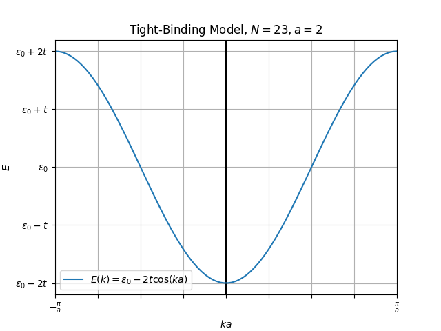
This expression is a simple sum over independent modes, each with a specific energy $ϵ_{k}$ . The function $ϵ_{k}$ is the energy-momentum dispersion relation, or band structure, of the non-interacting electrons. It tells us the energy of an electron as a function of its momentum.

The energy-momentum dispersion relation, $E(k) = \epsilon_0 - 2t\cos(ka)$, for a one-dimensional tight-binding model. This cosine band is the direct result of applying the Fourier transform to the nearest-neighbor hopping Hamiltonian. The width of the band is $4t$, determined by the hopping strength.

Conclusion

This lesson completes our journey through the fundamental principles of second quantization. You've learned the final, crucial technique for manipulating many-body Hamiltonians.

Here are the key takeaways:

Basis transformation is a key tool: Just as with classical coupled oscillators, changing to a basis that respects the symmetries of a quantum system can dramatically simplify the problem by decoupling the degrees of freedom.
The general rule is universal: Creation and annihilation operators transform as $d_{β}^{†} = \sum_{α} ⟨ α ∣ β ⟩ c_{α}^{†}$ , where the coefficients are simply the overlaps between the old and new single-particle basis states.
Fourier transform diagonalizes hopping: For a translationally invariant lattice, the transformation from the real-space site basis to the momentum basis is a discrete Fourier transform. This transformation converts the coupled nearest-neighbor hopping Hamiltonian into a simple, diagonal sum of energies for each momentum mode.
Band structure emerges naturally: The eigenvalues of the hopping Hamiltonian in the momentum basis, $ϵ_{k}$ , form the electronic band structure, a central concept in solid-state physics.

With these tools in hand, you are now fully equipped to tackle the models of correlated electron systems. In our next module, "The Tight-Binding Model," we will formally construct and analyze the non-interacting limit of the Hubbard model. You will use the basis change technique learned today to diagonalize the Hamiltonian, find the ground state, and calculate fundamental physical properties like electron density and kinetic energy.

Recommended resources

The Power of the Right Basis: An Analogy

General Transformation of Operators

Application: From Real Space to Momentum Space

Conclusion