Kinetic Energy and Band Filling

Welcome to the final lesson in our module on the tight-binding model. In our previous sessions, we have successfully constructed and diagonalized the Hamiltonian, defined the ground state by filling the single-particle energy levels up to the Fermi energy, and found that this ground state corresponds to a uniform electron density across the crystal lattice.

This lesson will complete our characterization of the non-interacting system. We will calculate the total energy of the ground state, which, in the absence of potential energy terms, is purely kinetic. This ground state kinetic energy is a fundamental quantity that depends on the band filling, and it will serve as a crucial reference point. When we later introduce the Coulomb interaction $U$ in the Hubbard model, the competition between this kinetic energy and the new potential energy will govern the physics of the system. Our goal is to evaluate this kinetic energy as a function of the band filling, $n$ .

The Ground State Energy

The total energy of the ground state $∣ Ψ_{0} ⟩$ is given by the expectation value of the Hamiltonian:

E_{k in} = ⟨ Ψ_{0} ∣ H^∣ Ψ_{0} ⟩

We use the diagonal, momentum-space representation of the tight-binding Hamiltonian, which you are now familiar with:

H^= k, σ \sum ϵ_{k} n^_{k σ} where ϵ_{k} = - 2 t cos (k a)

Since the ground state $∣ Ψ_{0} ⟩$ is an eigenstate of the number operators $n^_{k σ}$ , the calculation of the expectation value is direct. The operator simply returns the occupation number for each state $(k, σ)$ , which is either 1 (if occupied) or 0 (if empty).

E_{k in} = ⟨ Ψ_{0} k, σ \sum ϵ_{k} n^_{k σ} Ψ_{0} ⟩ = k, σ \sum ϵ_{k} ⟨ Ψ_{0} ∣ n^_{k σ} ∣ Ψ_{0} ⟩ = k, σ \sum ϵ_{k} ⟨ n^_{k σ} ⟩_{0}

At zero temperature ( $T = 0$ ), the ground state is formed by filling all states with energy $ϵ_{k}$ up to the Fermi energy $E_{F}$ . Therefore, the average occupation $⟨ n^_{k σ} ⟩_{0}$ is 1 for $ϵ_{k} \leq E_{F}$ and 0 for $ϵ_{k} > E_{F}$ .

The expression for the energy becomes a sum over all occupied states. Assuming a non-magnetic state, the occupations for spin-up and spin-down are identical, so we can sum over $k$ and multiply by 2:

E_{k in} = 2 occupied k \sum ϵ_{k}

The occupied $k$ -states are those within the Fermi sea, i.e., $∣ k ∣ \leq k_{F}$ , where $k_{F}$ is the Fermi momentum.

Calculation via k-space Integration

To evaluate this sum, we take the thermodynamic limit ( $N \to \infty$ ), where the discrete sum over $k$ becomes an integral. Recall the conversion rule for a 1D system of length $L = N a$ :

k \sum ⟶ \frac{L}{2 π} \int d k = \frac{N a}{2 π} \int d k

The total kinetic energy is then:

E_{k in} = 2 (\frac{N a}{2 π} \int_{- k_{F}}^{k_{F}} ϵ_{k} d k) = \frac{N a}{π} \int_{- k_{F}}^{k_{F}} (- 2 t cos (k a)) d k

The integral is straightforward to evaluate:

\int_{- k_{F}}^{k_{F}} (- 2 t cos (k a)) d k = - 2 t [\frac{sin ( k a )}{a}]_{- k_{F}}^{k_{F}} = - 2 t (\frac{sin ( k _{F} a ) - sin ( - k _{F} a )}{a}) = - \frac{4 t}{a} sin (k_{F} a)

Substituting this back, we find the total kinetic energy:

E_{k in} = \frac{N a}{π} (- \frac{4 t}{a} sin (k_{F} a)) = - \frac{4 N t}{π} sin (k_{F} a)

It is more convenient to work with the energy per site, $E_{k in} / N$ :

\frac{E _{k in}}{N} = - \frac{4 t}{π} sin (k_{F} a)

The final step is to express this energy as a function of the band filling, $n$ . We have previously established the relationship between $k_{F}$ and $n$ for a 1D chain:

k_{F} = \frac{nπ}{2 a}

Substituting this into our energy expression yields the final result:

\frac{E _{k in}}{N} (n) = - \frac{4 t}{π} sin (\frac{nπ}{2 a} \cdot a) = - \frac{4 t}{π} sin (\frac{nπ}{2})

This elegant formula gives the ground state kinetic energy per site for any filling $0 \leq n \leq 2$ .

Let's examine this result for a few key values of $n$ :

Empty band ( $n = 0$ ): $E_{k in} / N = - \frac{4 t}{π} sin (0) = 0$ . This is expected, as there are no electrons.
Half-filled band ( $n = 1$ ): $E_{k in} / N = - \frac{4 t}{π} sin (π /2) = - 4 t / π \approx - 1.27 t$ . The energy is minimized not at zero, but at a substantial negative value, reflecting the energy gained by electrons delocalizing across the lattice.
Full band ( $n = 2$ ): $E_{k in} / N = - \frac{4 t}{π} sin (π) = 0$ . A completely filled band also has zero total kinetic energy. While individual electrons are mobile, the band as a whole cannot carry a net current, and the sum of all single-particle energies $ϵ_{k}$ over the full Brillouin zone is zero.

Alternative View: The Density of States

There is a more general and powerful way to think about this calculation, using the concept of the Density of States (DOS), denoted $N (E)$ . The DOS counts the number of available single-particle states per unit energy, per site. For the 1D tight-binding model, it can be shown to be:

N (E) = \frac{1}{π 4 t ^{2} - E ^{2}} for ∣ E ∣ < 2 t

This function has divergences at the band edges $E = \pm 2 t$ , which are known as van Hove singularities.

Using the DOS, the band filling $n$ and the ground state energy per site are given by integrals over energy. We fill states up to the Fermi energy $E_{F}$ , so the integrals run from the bottom of the band ( $- 2 t$ ) up to $E_{F}$ . The factor of 2 accounts for spin.

n (E_{F}) = 2 \int_{- 2 t}^{E_{F}} N (E^{'}) d E^{'}

\frac{E _{k in}}{N} (E_{F}) = 2 \int_{- 2 t}^{E_{F}} E^{'} N (E^{'}) d E^{'}

These integrals can be solved to first find the relation between $n$ and $E_{F}$ , and then to find the energy $E_{k in} (n)$ . This method reproduces the exact same result we found with the k-space integration, but it highlights the central role of the density of states in determining the thermodynamic properties of the electron gas.

The following resource provides a concise guide to these calculations. Exercise 28 directly asks you to compute the average energy, which is what we have just done for the $T = 0$ case.

Elementary Introduction to the Hubbard Model

This guide by Richard Scalettar provides a set of clear exercises for the non-interacting (U=0) Hubbard model. It's a great way to solidify the formalism.

Focus on the section "VI. LIMIT OF NO INTERACTIONS". Review the definitions and the diagonalized Hamiltonian. Then, please read Exercise 28. This is precisely the calculation we have performed, expressed as a sum over Fermi-Dirac distributions. At zero temperature, the Fermi-Dirac distribution becomes a step function, and the sum becomes the integral we evaluated.

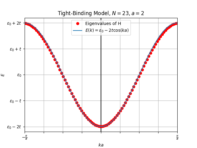
The plot below shows the analytical band structure $ϵ_{k} = - 2 t cos (k a)$ (blue line) that we have been using. The red dots represent the discrete energy eigenvalues of a finite chain. The ground state energy we calculated is the sum of the energies of all the red dots below the Fermi level.

The energy dispersion $E(k)$ for the 1D tight-binding model. The ground state kinetic energy is the sum of the energies of all occupied states, which lie on the blue curve between $-k_F a$ and $+k_F a$.

Conclusion

In this lesson, we have derived one of the most important results for the non-interacting electron system: the ground state kinetic energy as a function of band filling.

Key Takeaways:

The ground state energy is the sum of the single-particle energies of all occupied states.
In the 1D tight-binding model, the kinetic energy per site is given by the expression $E_{k in} / N = - \frac{4 t}{π} sin (\frac{nπ}{2})$ .
The energy is minimized at half-filling ( $n = 1$ ), not for an empty or full band. This energy gain is the driving force for electron delocalization.
The concept of the Density of States provides an alternative, powerful framework for calculating ground-state properties.

We have now completed our preliminary study of the tight-binding model. We understand its Hamiltonian, its band structure, its ground state, its charge distribution, and its energy. This non-interacting model provides the essential "stage" upon which the drama of electron-electron interactions will unfold.

Starting with the next lesson, we will introduce the on-site Coulomb repulsion, $U$ . This will take us from the tight-binding model to the full Hubbard model, where the interplay between kinetic energy ( $t$ ) and interaction energy ( $U$ ) gives rise to a rich spectrum of correlated electron phenomena, including the celebrated Mott transition.

Recommended resources

The Ground State Energy

Calculation via k-space Integration

Alternative View: The Density of States

Conclusion