Regimes of the Hubbard Model

The Landscape: Filling and the $U/t$ Ratio

Before we dive into the limits, we must define a crucial parameter: the filling, denoted by $\rho$ (or sometimes $n$). It is the average number of electrons per lattice site:

where $N_e$ is the total number of electrons and $N_s$ is the number of sites. Since each site can hold 0, 1, or 2 electrons, the filling ranges from $\rho =0$ (empty) to $\rho =2$ (completely full).

A particularly important case is half-filling, where $\rho =1$. Here, there is exactly one electron per site on average. In a simple band theory picture (which corresponds to $U=0$), this would mean the energy band is half-full, a quintessential feature of a metal. As we are about to see, the Hubbard model tells a very different story. The physics is governed by the interplay between filling and the dimensionless ratio $U/t$.

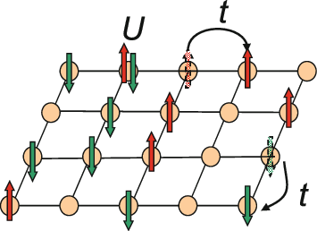
The Weak Coupling Regime ($U\ll t$): A Fermi Liquid

Let's begin in the regime where the interaction energy is a small perturbation to the kinetic energy. The simplest starting point is the extreme limit $U=0$.

When $U=0$, the Hubbard Hamiltonian reduces to the familiar tight-binding model:

As we saw in the previous module, this Hamiltonian is easily solved by Fourier transforming to momentum space. The eigenstates are Bloch waves with a well-defined dispersion relation $ϵ(\mathbf{k})$, and the many-body ground state is formed by filling these single-particle energy levels up to the Fermi energy, $E_F$, respecting the Pauli principle.

For any filling other than $\rho =0$ or $\rho =2$, there will be a finite density of states at the Fermi level, allowing for low-energy excitations. This is the definition of a metal.

When we introduce a small, non-zero $U$, the electrons can now scatter off one another. However, as long as $U\ll t$, the fundamental metallic nature of the system persists. The electrons are still delocalized, but their properties are modified. They acquire a finite lifetime and their effective mass may change. This state is known as a Fermi liquid.

Interestingly, even weak interactions can lead to dramatic collective phenomena. One such example is ferromagnetism, explained by the Stoner criterion. The argument, in essence, is a comparison of energy costs. Polarizing the spins (e.g., creating more spin-up than spin-down electrons) increases the total kinetic energy, because the majority-spin electrons are forced into higher-energy momentum states by the Pauli principle. However, polarization decreases the potential energy, since it reduces the chance of two opposite-spin electrons meeting on the same site. If the potential energy gain outweighs the kinetic energy cost, the system can spontaneously become ferromagnetic.

The following reading provides the derivation.

The Strong Coupling Regime ($U\gg t$): The Mott Insulator

Now let's turn to the opposite, and more fascinating, limit where $U\gg t$. Here, the cost of double occupancy is enormous, and the physics is dominated by the effort to avoid it.

The clearest picture emerges from the atomic limit, where we set $t=0$. The Hamiltonian becomes a simple sum over independent sites:

Each site has four possible energy eigenstates:

• Empty ($|0⟩$): Energy = 0
• Singly occupied ($|\uparrow ⟩$ or $|\downarrow ⟩$): Energy = 0
• Doubly occupied ($|\uparrow \downarrow ⟩$): Energy = $U$

Now, consider the case of half-filling ($\rho =1$). To minimize the total energy, the system will arrange itself to have exactly one electron on every site, completely avoiding any double occupancies. The ground state is massively degenerate, as any arrangement of spins (e.g., $|\uparrow ,\downarrow ,\uparrow ,\uparrow ,\downarrow ,\dots ⟩$) has the same energy, zero.

What happens if an electron tries to hop? It must move to an adjacent site, which, at half-filling, is already occupied. This would create an empty site and a doubly occupied site, at an energy cost of $U$. Because $U$ is large, this process is energetically forbidden. The electrons are effectively "frozen" in place. They cannot move to conduct electricity.

This is a Mott insulator: a material that should be a metal according to band theory (since its band is half-full) but is an insulator due to strong electron-electron repulsion.

The following reading gives a clear and quantitative description of this limit.

The transition from a metal at small $U$ to a Mott insulator at large $U$ can be beautifully visualized by looking at the evolution of the density of states.

Superexchange: The Origin of Antiferromagnetism

In the strong-coupling, half-filled ground state, we have a lattice of localized spins. The hopping term $t$, while small, is not zero. When treated as a perturbation, it has a profound effect: it lifts the massive spin degeneracy and dictates how the localized moments should align.

Consider two adjacent sites with single electrons.

• Case 1: Antiparallel spins ($\uparrow ,\downarrow$). The spin-up electron can virtually hop to the adjacent site, creating a temporary doubly occupied state ($0,\uparrow \downarrow$) with high energy $U$. It can then hop back. This virtual process is allowed by the Pauli principle. Second-order perturbation theory tells us that this process lowers the energy of the antiparallel configuration by an amount proportional to $-t^2/U$.
• Case 2: Parallel spins ($\uparrow ,\uparrow$). The spin-up electron cannot hop to the adjacent site, as that site already contains a spin-up electron. This process is forbidden by the Pauli principle.

The net result is that having antiparallel spins on neighboring sites is energetically favorable. This effective interaction, mediated by virtual hopping through a high-energy state, is called superexchange. It leads to an effective low-energy Hamiltonian for the spins that is equivalent to the Heisenberg antiferromagnetic model, with an exchange coupling $J\approx 4t^2/U$.

This is one of the most important results of the Hubbard model: in the strong coupling limit at half-filling, it naturally explains the emergence of antiferromagnetism. A concrete way to see this is by solving the simplest non-trivial system: the two-site Hubbard model.

Conclusion

In this lesson, we have mapped out the basic phase diagram of the Hubbard model as a function of the interaction strength $U/t$, with a special focus on the half-filled case.

Key Takeaways:

• Weak Coupling ($U\ll t$): The system behaves like a metal, albeit one where electrons interact. Its properties can be described by Fermi liquid theory. For a high density of states at the Fermi level, this weak repulsion can even drive a transition to a ferromagnetic state (Stoner instability).
• Strong Coupling ($U\gg t$): At half-filling, the system becomes a Mott insulator. The large energy cost of double occupancy localizes electrons, opening a charge gap of order $U$. The single metallic band splits into lower and upper Hubbard bands.
• Half-Filling and Magnetism: In the strong-coupling, half-filled regime, virtual hopping processes give rise to an effective antiferromagnetic interaction between localized spins. This superexchange mechanism, with coupling $J\sim t^2/U$, explains why so many Mott insulators are also antiferromagnets.

You now have a conceptual framework for the major physical regimes of the Hubbard model. We've touched upon concepts like spin and magnetic ordering, which depend on the symmetries of the Hamiltonian. In our next lesson, we will formalize this by exploring the key symmetries of the Hubbard model, starting with SU(2) spin-rotation symmetry.