Introduction
In our last lesson, we built the "immune system" for our model by implementing a robust, centralized error-checking framework. A model that is mathematically sound is essential, but for it to be truly powerful, it must also be flexible. This brings us to the topic of this lesson: constructing the model's "skeleton"—a dynamic timeline.
Today, we will move beyond static, hard-coded structures to build a timeline that can adapt to changing assumptions and time horizons. You will learn to create a model architecture that cleanly separates historical data ("Actuals") from projected data ("Forecasts") and allows for seamless updates. For both your AFM exam preparation and real-world startup modeling, the ability to easily extend a forecast, change its periodicity, or roll it forward with new monthly actuals is a non-negotiable skill. Your experience in data modeling and ETL design will be particularly relevant as we explore how to map and integrate historical data streams into the forecast structure.
By the end of this lesson, you will be able to build a flexible timeline driven by a handful of inputs, using date functions and control flags to manage different time periods dynamically.
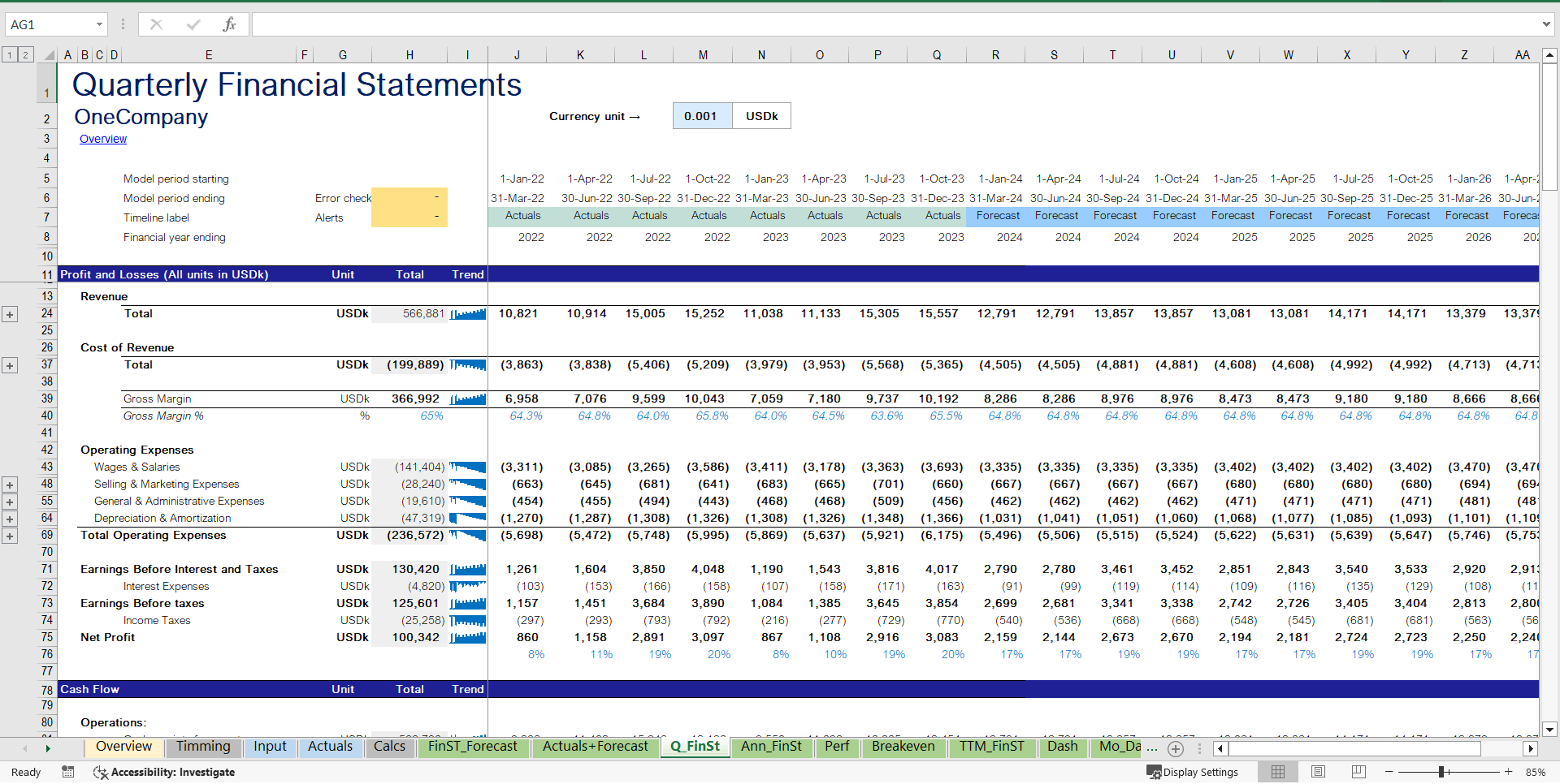
The Foundation: Core Timeline Inputs and Calculations
A dynamic timeline begins not in the columns of your financial statements, but on a dedicated inputs or control sheet. Instead of typing dates manually across the top of your model, we will drive the entire timeline from a few key inputs. This principle is central to building scalable and maintainable models.
Let's begin by understanding the core components and the Excel functions used to build them.
8 Financial Modeling Best Practices for 2025
This article from Finzer provides an excellent overview of why a dynamic timeline is a best practice. Focus on Section 5, "Dynamic Timeline and Scalable Periods".
Pay close attention to the concepts under The Flow of Information, which describes the foundational setup, and the specific functions mentioned in the Actionable Tips. This will set the stage for the practical implementation to follow.
As the article highlights, the key is to have a dedicated section for timeline inputs (e.g., Model Start Date, Forecast Start Date) and then use formulas to generate all date-related rows.
The following video provides a fantastic, hands-on demonstration of how to build these rows from scratch. The presenter, Danielle Stein Fairhurst, is an FMI expert, and her methods align directly with the standards you'll encounter in the AFM exam.
Modelling Timelines with Dynamic Array Functions in Excel (Part 1 of 5)
This video, "Modelling Timelines with Dynamic Array Functions in Excel," will walk you through the key formulas.
Watch the following segments to see how a complete timeline is constructed: Period Counter: Note the use of the SEQUENCE function to create a dynamic counter. This is a modern approach, but the principle is the same as a simple =IF(previous_cell < total_periods, previous_cell+1, 0). Start and End Dates: See how EOMONTH is used with the counter to create the period-end dates, and how subsequent period-start dates are derived. The use of IF statements to show blank cells beyond the model's horizon is a key technique for keeping the model clean. Helper Rows: Observe the creation of rows for Year, Month, and the number of days in the period. These will be indispensable for calculations like revenue seasonality, interest, and depreciation.
To summarize the process shown in the video, a best-practice timeline typically includes these rows, all driven by formulas:
- Period Counter: A simple
1, 2, 3...across the columns of your model. - Period End Date: Calculated using
EOMONTH(Model_Start_Date_Input, Period_Counter - 1). - Period Start Date: Calculated as
EOMONTH(Previous_End_Date, -1) + 1for the first period, and simplyPrevious_End_Date + 1for subsequent periods. - Helper Calculations: Rows for
YEAR(End_Date),MONTH(End_Date), and(End_Date - Start_Date) + 1to get the number of days in the period, which correctly accounts for leap years.
Distinguishing History from Forecast: Timeline Flags
With the basic date structure in place, the next step is to make the model "aware" of which periods are historical and which are forecasts. We achieve this using flags, which are simple binary rows of 1s and 0s (or TRUE/FALSE) that control logic throughout the model.
The most fundamental flag is the Forecast Period Flag. If you have an input cell named Forecast_Start_Date, the formula in your flag row would be:
=IF(Period_End_Date >= Forecast_Start_Date, 1, 0)
This formula will place a 0 in all historical columns and a 1 in all forecast columns. You can then create a Historical Period Flag with the formula =1 - Forecast_Period_Flag.
These flags are incredibly powerful. They are used inside IF functions to switch the model's logic. For any given line item, the formula structure becomes:
=IF(Forecast_Period_Flag=1, [Formula for Forecast], [Link to Actuals])
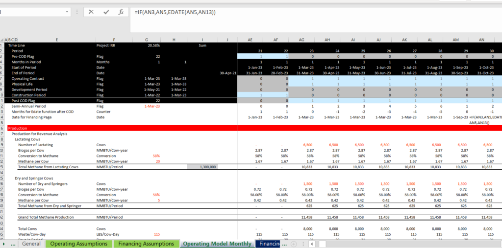
This single line of logic is the engine of a rolling forecast. The image below, from a project finance model, shows a more complex set of flags used to manage different operational phases. The principle is identical: using 1s and 0s to control calculations period by period.
Building a Rolling Forecast: Mapping and Integrating Actuals
Now, let's address the [Link to Actuals] part of our IF statement. A naive approach would be to manually copy-paste historical data each month. A robust, professional approach automates this process. Your background in ETL and data management will be very useful here. We essentially perform a mini-ETL process within Excel.
The key is to create a "mapping" system that connects the raw data from your accounting system to the line items in your financial model. The following video demonstrates this powerful technique perfectly.
Mapping Actuals to a Rolling Forecast
This video, "Mapping Actuals to a Rolling Forecast," shows a clean and scalable method for integrating historical data.
Watch from the beginning to understand the concept of creating a "mapping" column in your actuals data tab. From the formula demonstration, focus on how the SUMIFS function is used in the main model to pull the correct data for the correct period. Finally, note the benefits of this approach, particularly how it handles new accounts without breaking your model.
The core formula pattern demonstrated in the video, adapted for our purpose, looks like this:
=SUMIFS(Actuals_Value_Column, Actuals_Date_Column, Period_End_Date_Header, Actuals_Mapping_Column, Model_Line_Item_Name)
By combining this SUMIFS formula with our forecast flag, we arrive at a complete, dynamic formula for each line item in our Profit & Loss statement:
=IF(Forecast_Period_Flag=1, [Forecast Logic], SUMIFS(...))
When you get new monthly actuals, you simply paste them into your data tab, ensure they are mapped, and extend the Forecast_Start_Date input by one month. The model automatically "rolls" forward, with the new month pulling from SUMIFS and the old first forecast month now also pulling from SUMIFS.
Advanced Timeline Structures and Best Practices
To elevate your models to a professional standard, it's worth considering a few more advanced techniques and best practices, as detailed by expert modeler Edward Bodmer.
Flexible Timelines in Project Finance Models – Edward Bodmer – Project and Corporate Finance
This article provides a masterclass in building truly flexible timelines, drawing on examples from project finance.
As you read, focus on these key ideas: Master Timeline: The concept of having a single, consistent timeline across all sheets. Timeline at the Top: Reinforces the best practice of placing all date and flag rows at the top of every calculation sheet for consistency. Notice the critique of models that fail to do this. Avoid Hard-Coding: This section shows a dramatic example of what not to do—hard-coding years into formulas renders a model inflexible. Handling Fiscal Years: Skim this section to understand the logic for creating fiscal year counters that differ from the calendar year, using EDATE and MONTH functions. This is a hallmark of an advanced modeler.
Conclusion
In this lesson, we have designed and built the structural skeleton of our model: a dynamic timeline. You've learned that by driving all time-based calculations from a few key inputs and using flags, you can create a flexible and easily maintainable model that cleanly separates historicals from forecasts.
Here are the key takeaways:
- Centralize Inputs: A dynamic timeline is driven by inputs like a
Model Start DateandForecast Start Date, which should live on a dedicated control sheet. - Use Date Functions: Build your timeline rows using Excel's date functions (
EOMONTH,EDATE,YEAR,MONTH) to ensure accuracy and flexibility. - Leverage Flags: Use binary flags (rows of 1s and 0s) to make the model "aware" of the period type (e.g., historical vs. forecast, construction vs. operation).
- Automate Actuals Integration: Implement a
SUMIFS-based mapping system to pull historical data into your model automatically, creating a true "rolling forecast." - Maintain Consistency: Place the timeline block (dates and flags) at the top of every relevant worksheet in your model to ensure consistency and readability.
We have now established the basic flags for our timeline structure. In our next lesson, we will expand on this powerful concept by building a dedicated controls sheet. This sheet will house not just our timeline inputs, but also a more sophisticated set of flags and switches that will allow us to toggle between different scenarios—such as base, upside, and downside cases—across the entire model.