Redshift Cluster Design & Node Selection

1. The Architecture of a Modern Data Warehouse

Amazon Redshift is a fully managed, petabyte-scale data warehouse service. Unlike a traditional transactional database (like PostgreSQL or MySQL), which is optimized for quick row-based reads and writes (OLTP), Redshift is designed for Online Analytical Processing (OLAP). This means it's built to execute complex queries over vast amounts of data very quickly.

It achieves this speed through two core architectural principles:

• Columnar Storage: Data is stored in columns, not rows. For analytical queries that often aggregate a few columns (e.g., SUM(sales)), this is incredibly efficient because the system only reads the data for those specific columns, drastically reducing I/O.
• Massively Parallel Processing (MPP): Queries are broken down and executed in parallel across a cluster of nodes. This "divide and conquer" approach allows Redshift to leverage the combined compute power and I/O bandwidth of all nodes in the cluster.

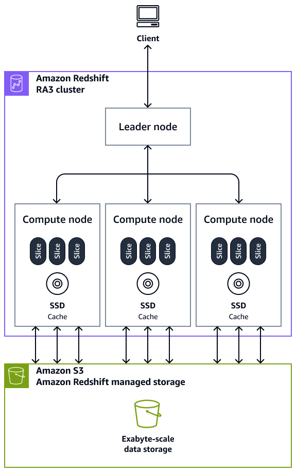
A Redshift cluster consists of two main components: a Leader Node and one or more Compute Nodes.

• Leader Node: This is the brain of the operation. Your client application (e.g., a SQL client or BI tool) connects to the leader node. It receives your query, parses it, develops an optimized query execution plan, and compiles code.
• Compute Nodes: These are the workhorses. The leader node distributes the compiled code to the compute nodes, which execute the query in parallel on the portion of data they store locally. They then send their partial results back to the leader node for final aggregation before the result is returned to you.

To see this architecture explained visually, let's watch a short clip.

The diagram below illustrates the modern architecture for an RA3 Redshift cluster, which we will explore in the next section. Notice how compute nodes have their own local SSD cache but also leverage Amazon S3 for durable, scalable storage.

2. Choosing the Right Node Type: RA3 vs. DC2

When you provision a Redshift cluster, your most important decision is the node type. This choice dictates the CPU, RAM, and, crucially, the storage architecture of your cluster. For the exam, you need to know the two primary node families: DC2 and RA3.

Let's start by reading the official AWS documentation, which provides the definitive guide to these node types.

To summarize the key distinction:

• DC2 (Dense Compute):

  • Architecture: Compute and storage are tightly coupled. Each node has local, high-performance NVMe SSD storage.
  • Scaling: To increase storage, you must add more nodes, which also increases your compute cost.
  • Best For:
    • Performance-critical workloads with datasets under 1 TB (compressed).
    • Situations where data size is stable and predictable.
    • Offers the best performance for its price at smaller scales.

• RA3 (with Managed Storage):

  • Architecture: Compute and storage are decoupled. It uses large, high-performance SSDs on each node as a cache, while the full dataset is durably stored in Amazon S3 (this is called Redshift Managed Storage).
  • Scaling: You can scale compute and storage independently. You size your cluster for the query performance you need (number of nodes), and the managed storage automatically scales as your data grows.
  • Best For:
    • Large datasets (typically >1 TB) or those expected to grow significantly.
    • Workloads where compute and storage requirements scale at different rates.
    • When you want to take advantage of modern Redshift features like data sharing and AQUA (Advanced Query Accelerator).

For most modern data warehousing use cases, RA3 is the recommended node type due to its flexibility and scalability.

3. A Practical Guide to Sizing Your Cluster

Once you've chosen a node type, you need to determine the size—that is, which specific instance (.xlplus, .4xlarge, etc.) and how many nodes.

Here's a straightforward methodology for estimating your initial cluster size.

Let's formalize that sizing methodology:

1. Estimate Uncompressed Data Size: Start with the total size of the source data you plan to load into Redshift.
2. Apply Compression: Redshift automatically compresses data. A conservative estimate is a 3x to 4x compression ratio. So, divide your uncompressed data size by 3.
3. Add Headroom: You should always leave free space for intermediate query processing, temporary tables, and future data growth. A good rule of thumb is to aim for a cluster that is no more than 70-80% full. This means adding a 20-30% buffer to your compressed data size.
4. Select Node Configuration: Using the final estimated storage requirement, consult the node specification tables to find a combination of node type and count that meets your needs.

Example Calculation

Let's say you need to build a data warehouse for 30 TB of uncompressed source data.

1. Uncompressed Size: 30 TB
2. Compressed Size: 30 TB / 3 = 10 TB
3. Add Headroom: 10 TB * 1.25 = 12.5 TB (adding a 25% buffer)
4. Select Nodes: Now, you look for a configuration that provides at least 12.5 TB of storage.

To do this, you'll need the detailed node specifications.

Continuing our example, let's consider the ra3.4xlarge node. Each node has a managed storage limit of 128 TB, which is far more than our 12.5 TB requirement. With RA3, the decision is more about performance than storage capacity. We might start with the smallest recommended cluster (2 nodes) and monitor performance.

If we were considering DC2 nodes, the calculation is more direct. The dc2.8xlarge has 2.56 TB of local storage.

• 12.5 TB / 2.56 TB per node ≈ 4.88 nodes.
• Since you can't have a fraction of a node, you would round up to 5 dc2.8xlarge nodes.

Practical Tools for Sizing

For the exam, you should also be aware of the tools AWS provides to simplify this process.

• "Help me choose" Sizing Calculator: A simple wizard in the AWS console that gives you a recommended starting configuration based on your data size and query patterns. This is often the best starting point.
• Node Configuration Comparison Utility: A more advanced tool for running performance benchmarks across different cluster configurations to find the optimal price/performance for your specific workload.

4. Production-Ready Architecture: HA and Scalability

Finally, designing a production cluster involves more than just sizing. You must also consider high availability and future scalability.

• High Availability (HA): A Redshift cluster with two or more compute nodes will automatically mirror data across nodes. If one node fails, Redshift can continue operating from the replica data on another node, minimizing downtime. Single-node clusters are not recommended for production workloads as they represent a single point of failure.
• Scalability: Your cluster needs will change over time. Redshift supports cluster resizing to add or remove nodes. This is another area where RA3 shines, as its decoupled architecture makes resizing operations faster and less disruptive than with DC2, especially when only compute needs to change.

Conclusion

In this lesson, you have learned the essential principles for designing an Amazon Redshift cluster architecture. This is a foundational skill for any data engineer working with AWS and a frequent topic on the certification exam.

Key Takeaways:

• Redshift's speed comes from its MPP architecture and columnar storage.
• A cluster consists of a single Leader Node for query planning and multiple Compute Nodes for parallel execution.
• The primary node families are DC2 (coupled storage/compute) and RA3 (decoupled storage/compute). RA3 is the modern, flexible choice for most workloads, especially those with growing data.
• A practical sizing methodology involves estimating compressed data size, adding a buffer, and selecting a node configuration that meets your storage and performance needs.
• For production, always use a multi-node cluster (at least 2 nodes) for high availability.

Next Up:
Now that we understand how to provision the cluster's physical infrastructure, our next lesson will focus on optimizing the logical data structure within it. We will learn how to "Implement optimal table design using distribution styles and sort keys," which are critical techniques for maximizing query performance in a distributed environment.