Understanding Residuals

Welcome! In our last lesson, we focused on how to combine the interpretations of the intercept and slope into a single, cohesive statement about the entire regression model. We also briefly introduced the concept of a residual as a measure of prediction error.

Today's lesson is a focused, practical drill on that exact topic. Mastering residuals is non-negotiable for your exam, as they are the building blocks for almost all model diagnostics. We will solidify the definition, practice the calculation until it's second nature, and ensure you can interpret any residual's meaning instantly. This session fully covers the last component of our first module, defining a residual as the difference between an observed and predicted value.

What is a Residual? The Core Idea

Before we jump into formulas, let's establish a strong intuition. A residual is, quite simply, what's "left over" after your model makes a prediction. The video below offers a great real-world analogy to anchor this idea.

Statistics 101: Linear Regression, Residual Analysis

In this clip from his "Statistics 101" series, Brandon Foltz provides an excellent intuitive definition of a residual before giving the formal statistical one.

Watch the segment from this video. Pay attention to the paycheck analogy he uses—it perfectly captures the concept of a residual as the amount "left over". Then, see how he translates this into the statistical definition: the difference between an observed value and the value predicted by the model.

The Formal Definition and Formula

Building on that intuition, the formal definition is direct and crucial to memorize. A residual ( $e$ ) is the observed value ( $y$ ) minus the predicted value ( $y^$ ).

e = y - y^

It's the vertical distance from an actual data point to the regression line on a scatter plot. The following reading formalizes this and clarifies how to interpret the sign of the residual.

7.2: Line Fitting, Residuals, and Correlation - Statistics LibreTexts

This excerpt from Statistics LibreTexts provides a clear, concise definition and visual representation of residuals.

Please read the section titled "Residuals". Focus on three key points: The formula: e_i = y_i - \hat{y}_i. The concept that a residual is the vertical distance from the observation to the line. The rule for the sign: positive residuals are for points above the line, and negative residuals are for points below it.

To summarize the key interpretation rule:

Positive residual ( $e > 0$ ): The model under-predicted the actual value ( $y > y^$ ). The data point is above the regression line.
Negative residual ( $e < 0$ ): The model over-predicted the actual value ( $y < y^$ ). The data point is below the regression line.

Calculation Drill: An Exam-Style Problem

Let's apply this to a typical exam question. You are given a scenario, a regression equation, and a specific data point. Your task is to calculate the residual.

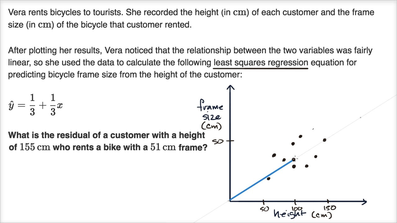
A scatter plot shows the relationship between customer height and bicycle frame size, with a least-squares regression line drawn. The problem asks for the residual for a specific customer.

Let's solve this step-by-step, just as you would in the exam.

1. Identify Given Information:

Predictor variable ( $x$ ): Customer height = 155 cm
Observed response ( $y$ ): Rented bike's frame size = 51 cm
Regression Equation: $y^= \frac{1}{3} + \frac{1}{3} x$

2. Calculate the Predicted Value ( $y^$ ):
Substitute the customer's height ( $x = 155$ ) into the equation to find the frame size the model predicts.

y^= \frac{1}{3} + \frac{1}{3} (155) = \frac{1}{3} + \frac{155}{3} = \frac{156}{3} = 52 cm

3. Calculate the Residual ( $e$ ):
Now, apply the formula $e = y - y^$ .

e = 51 - 52 = - 1 cm

4. Interpret the Result (Exam-Style Answer):
The residual is -1 cm. This means for a customer with a height of 155 cm who rented a 51 cm frame, the model over-predicted the frame size by 1 cm.

Visualizing Residuals and the Residual Plot

So far, we've thought of residuals as vertical lines on a scatter plot. However, for diagnosing model problems, we use a specialized chart: the residual plot.

A residual plot "flattens" the regression line to be horizontal at y=0 and plots the residual for each data point against its corresponding predicted value. This makes it much easier to spot patterns in the errors.

This is a standard residual vs. fitted values plot. The y-axis shows the residuals, and the x-axis shows the predicted (fitted) values from the model. The horizontal line at 0 is the baseline.

For now, the key takeaway is what this plot represents. For a well-behaved model, you want to see a random, "shotgun blast" pattern of dots scattered around the zero line, with no obvious shapes or trends. In Module 4, we will use plots like this to diagnose major problems like non-linearity and heteroscedasticity.

Practice Drill

Now it's your turn. Use the same step-by-step process.

Given Information:

A company uses a regression model to predict an employee's monthly sales (Sales, in thousands of dollars) based on their years of experience (Experience).
The regression equation is: Sales = 10 + 2.5 * Experience
An employee with 8 years of experience had actual sales of $28,000 last month.

Your Task:

Calculate the predicted sales for this employee.
Calculate the residual.
Write a one-sentence interpretation of the residual.

Solution

Identify Information:
- $x = 8$ years
- $y = 28$ (in thousands of dollars)
- Equation: $y^= 10 + 2.5 x$
Calculate Predicted Value ( $y^$ ):
$y^= 10 + 2.5 (8) = 10 + 20 = 30$
The predicted sales are $30,000.
Calculate Residual ( $e$ ):
$e = y - y^= 28 - 30 = - 2$
The residual is -2 (in thousands of dollars).
Interpretation:
- Answer: The model over-predicted this employee's sales by $2,000.

Conclusion

This focused drill completes our first module. You are now equipped with the foundational skills for interpreting the output of a simple linear regression model.

Key Takeaways for Your Exam:

Residual Definition: A residual is the error in a single prediction, calculated as the observed value minus the predicted value ( $e = y - y^$ ).
Calculation: First, use the regression equation to find the predicted value $y^$ for a given $x$ . Then, subtract this from the actual observed value $y$ .
Interpretation: A positive residual means the model under-predicted. A negative residual means the model over-predicted. The absolute value of the residual indicates the magnitude of the prediction error.

In the next module, we will move from analyzing individual errors to assessing the overall performance of the entire model. We'll ask, "How good is the model as a whole?" and answer this question using two critical statistics: R-squared and the Residual Standard Error.