Welcome to our first lesson on diagnosing model assumptions. In the previous module, we focused on assessing the overall significance of our model with the F-test. We learned how to determine if our model has predictive power. Now, we shift our focus to a different but equally crucial question: is our model valid?
A linear regression model is built on a foundation of several key assumptions. If these assumptions are violated, our model's predictions and the conclusions we draw from it can be unreliable. In this module, we'll become detectives, using diagnostic plots to check for evidence of these violations.
Today's lesson focuses on the first and most fundamental assumption: linearity. You will learn how to use the single most important diagnostic tool—the residual vs. fitted plot—to determine if the linear relationship you've modeled is truly appropriate for your data.
The Logic of Residual Plots
Before we dive in, let's quickly re-establish what residuals and fitted values are, as they are the building blocks of our diagnostic plots.
- Fitted Value (): This is the prediction your model makes for a given observation. It's the value that falls on the regression line.
- Residual (): This is the model's error for that observation, calculated as the actual value minus the fitted value ().
The core idea of residual diagnostics is simple: if your model is a good fit for the data, the errors (residuals) should be random and have no pattern. A residual plot helps us see if any patterns exist. For this lesson, we will focus on the Residuals vs. Fitted Plot, which is the primary tool for checking the linearity assumption.
- X-axis: Fitted values ()
- Y-axis: Residuals ()
What to Look For: The Good and the Bad
Your job is to look for patterns in this plot. There are two main scenarios you will encounter.
1. The Ideal Plot: Random Scatter
When the linearity assumption holds, the Residuals vs. Fitted plot should look like a random cloud of points scattered evenly around the horizontal line at Residual = 0. There should be no discernible shape or trend.

A "good" plot tells you that the errors of your model are not related to the size of the predicted value. This supports the conclusion that a linear model is a reasonable choice. The video below provides a great narration of what to hope for in a residual plot.
Simple Linear Regression: Checking Assumptions with Residual Plots
This video from jbstatistics explains and illustrates what an ideal residual plot looks like.
Watch the segment from this clip where the narrator describes a "random scattering of points" and explains why this indicates no problems with the model assumptions.
2. The Problem Plot: Curvature
The most common sign of a non-linear relationship is a clear, systematic pattern in the residuals. Most often, this will appear as a curve or U-shape.
Look again at the image of the three plots. The plot on the right, labeled "Nonlinear," shows a distinct curve. This means the model is systematically making errors: it under-predicts for small and large fitted values (residuals are positive) and over-predicts for mid-range values (residuals are negative). This is a dead giveaway that the relationship you are trying to model is not linear.
This excellent article from Statology walks through a perfect example of this problem.
How to Interpret a Curved Residual Plot (With Example)
This article demonstrates what happens when you fit a linear model to data that is actually quadratic.
Read the section Example: Interpreting a Curved Residual Plot. Pay close attention to the first residual plot shown, which has a clear curved pattern. The text explains that this pattern indicates that a linear model is not a good fit.
When you see a curve, the linearity assumption is violated. Your straight-line model is failing to capture the true underlying shape of the data. The following video provides a powerful visual demonstration of this exact issue.
Checking Linear Regression Assumptions in R | R Tutorial 5.2 | MarinStatsLectures
This video from MarinStatsLectures shows a non-linear dataset, the incorrect linear model fit to it, and the resulting curved residual plot.
Watch the segment from this demonstration. Notice how the U-shaped pattern in the residual plot directly reflects the inadequacy of the straight line seen in the scatter plot.
Exam-Style Interpretation
For your exam, you need to be able to state your conclusion clearly and concisely.
-
If the plot looks good (random scatter):
The residual vs. fitted plot shows a random scatter of points around the zero line with no discernible pattern. This supports the assumption that the relationship is linear.
-
If the plot looks bad (curved pattern):
The residual vs. fitted plot shows a clear curved (or U-shaped) pattern. This violates the linearity assumption, indicating that a linear model is not appropriate for this data.
Why This Plot is Essential
You might wonder, "Can't I just look at a scatter plot of Y vs. X?" You can, and you should for simple linear regression. However, the residual plot is a more powerful and essential tool, especially in multiple linear regression. With multiple predictors, you cannot create a single scatter plot to see the overall relationship. The residual vs. fitted plot condenses all that information into one graph, allowing you to assess the model's linearity regardless of how many predictors you have.
Practice Drill
Examine the following residual vs. fitted plot.
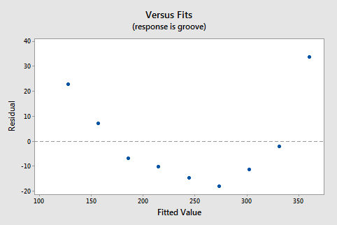
Your Task:
What does this plot tell you about the model's linearity assumption? Write a one-sentence, exam-style conclusion.
Solution
Exam-Style Conclusion:
The residual vs. fitted plot shows a clear U-shaped pattern, which indicates that the linearity assumption is violated and the linear model is not appropriate for this data.
Conclusion
You have now learned how to perform the first critical diagnostic check on a regression model. By examining the residual vs. fitted plot, you can confidently assess the linearity assumption.
Key Takeaways:
- The residual vs. fitted plot is your primary tool for checking the linearity assumption.
- A random, formless cloud of points around zero is good. It means the linearity assumption holds.
- A distinct pattern, especially a curve or U-shape, is bad. It means the linearity assumption is violated, and your model is likely misspecified.
In our next lesson, we will continue our detective work using the very same plot. We will ignore the shape of the points and instead focus on their spread to diagnose another potential problem: heteroscedasticity, or non-constant variance.