Welcome back. In our last session, we built a comprehensive playbook for writing precise, exam-style interpretations of regression outputs. You now have templates for explaining coefficients, model fit, and diagnostic plots. Now, we move to the final piece of the puzzle before our full review: defense. Your exam will be designed to test not just what you know, but also your ability to avoid common statistical fallacies and misinterpretations.
This lesson is dedicated to identifying and sidestepping the most common exam traps. Mastering these will help you secure the highest marks by demonstrating a deeper, more critical understanding of linear regression. We'll focus specifically on the pitfalls of confusing correlation with causation and the several ways that dummy variables can be mishandled.
1. Trap: "Correlation Implies Causation"
This is perhaps the most fundamental error in statistics and a very common trap on exams. A regression model built on observational data can show a strong association between variables, but it cannot, by itself, prove that one variable causes the other.
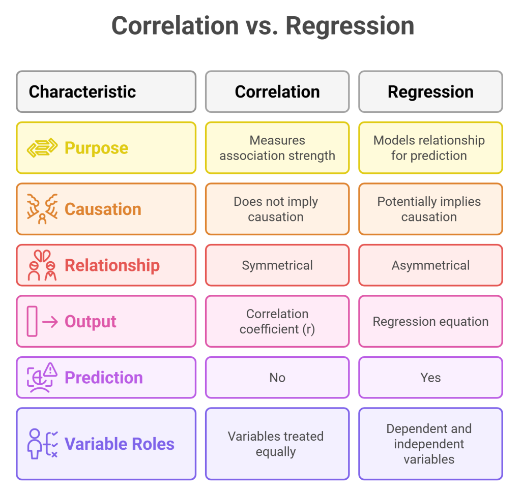
A high and a significant p-value for a predictor do not give you license to use causal language. There could be a third, unobserved variable (a "lurking" or "confounding" variable) that is driving both.
To understand this intuitively, watch this short video.
Correlation vs Causation (Statistics)
This video provides a classic and memorable example to distinguish correlation from causation.
Watch the segments introducing the concept and the ice cream example. The key insight is understanding the role of the sun as a confounding variable that affects both ice cream sales and sunburns.
How to Avoid the Trap:
Your language is your defense. In the previous lesson, we emphasized using cautious wording. Here is a direct comparison to make it crystal clear:
-
WRONG (Causal Language):
- "Increasing advertising by $1,000 causes sales to increase by 500 units."
- "This proves that more study time leads to higher grades."
-
CORRECT (Associational Language):
- "An increase in advertising of $1,000 is associated with an average increase of 500 units in sales."
- "The model predicts that for each additional hour of study time, grades are expected to increase by [β₁] points, on average."
On your exam, always default to associational language unless the problem explicitly states the data comes from a randomized controlled experiment.
2. Trap: Mishandling Dummy Variables
Dummy variables are essential for including categorical predictors in a model, but they come with two major traps: misinterpreting the coefficient and the "dummy variable trap."
A) Misinterpreting the Dummy Coefficient
A common mistake is to interpret the coefficient of a dummy variable in isolation. Remember, the coefficient represents a change in the intercept or the difference in the average response relative to the omitted base category.

Let's watch a video that walks through this with a concrete example.
This video on dummy variables clearly explains how to interpret the coefficients in the context of a gender pay gap example.
Pay close attention to the section from the interpretation of the coefficients. Notice how the intercept (\beta_0) represents the average income for the base category (males, where female=0), and the dummy coefficient (\beta_1) is the difference in average income for the other category (females, where female=1).
How to Avoid the Trap:
Your interpretation must always reference the base category.
- Model:
Salary = 50000 + 10000 * Urban(whereUrban=1 for urban, 0 for rural) - WRONG: "The Urban coefficient is 10,000." (This says nothing).
- WRONG: "Urban employees earn $10,000." (No, that's the difference).
- CORRECT: "Holding other predictors constant, the predicted salary for an employee in an urban location is, on average, $10,000 higher than for an employee in a rural location (the base category)."
B) The Dummy Variable Trap
If a categorical variable has k levels, you must only include k-1 dummy variables in the model. If you include k dummy variables, the model will fail because of perfect multicollinearity. The set of dummy variables will perfectly predict the intercept.
For example, if you have a Season variable with 4 levels (Winter, Spring, Summer, Autumn), you should only include 3 dummy variables (e.g., is_spring, is_summer, is_autumn). The base case, where all three are 0, would be Winter.
The following resource explains this very clearly.
Dummy Variables in Regression - Statistics and Probability
This article from StatTrek provides a direct and practical warning about a technical mistake known as the dummy variable trap.
Read the section titled Avoid the Dummy Variable Trap. It explains precisely why including a dummy for every category creates a redundancy that makes the model impossible to solve.
How to Avoid the Trap:
This is a rule to memorize: Always use k-1 dummy variables for a categorical variable with k levels. When you see a categorical variable in an exam problem, immediately count its levels and confirm the model is using the correct number of dummy variables.
3. Other Common Traps
Beyond the two major traps above, a few other common errors can cost you marks.
- Trap: Interpreting Non-Significant Coefficients. If a predictor's p-value is greater than your significance level (e.g., p > 0.05), you cannot interpret its coefficient. The data does not provide enough evidence to conclude that a relationship exists.
- How to Avoid: If p > 0.05, your conclusion should be: "There is no statistically significant evidence of a linear relationship between [X variable] and [Y variable] at the 5% significance level." Do not discuss the coefficient's value. The resource
Interpreting Regression Coefficientsmakes this point forcefully.
Common Mistakes in Interpretation of Regression Coefficients
This resource from the University of Texas at Austin highlights subtle but critical mistakes in interpretation.
Focus on point #3, interpreting a non-significant coefficient. This is a classic error that's easy to avoid once you're aware of it.
- Trap: Ignoring "Holding Others Constant" in MLR. We covered this in the last lesson, but it's worth repeating. Omitting this phrase when interpreting a coefficient in a multiple regression model is a critical error.
- How to Avoid: Burn the phrase "Holding all other variables constant..." into your memory. Always use it at the start of your interpretation for any coefficient in an MLR model.
Practice Drill: Spot the Trap!
For each statement below, identify the trap and explain the error in one sentence.
- A model predicts student
exam_scorefromhours_studiedandattended_tutoring(1 if yes, 0 if no). The output forattended_tutoringisEstimate = 5.2, p-value = 0.02. The interpretation given is: "Students who attended tutoring scored 5.2 points." - A regression of house prices on several features finds that the coefficient for
num_bathroomsis 25,000 with a p-value of 0.34. An analyst reports: "Each additional bathroom is associated with an increase of $25,000 in price, but the effect is not statistically significant." - A study finds a strong positive correlation between the number of firefighters at a fire and the amount of damage caused. The conclusion drawn is: "To reduce damage, we should send fewer firefighters."
Solution
- Trap: Misinterpreting a dummy coefficient. The error is that 5.2 is the additional score associated with attending tutoring compared to not attending; it is not the total score.
- Trap: Interpreting a non-significant coefficient. The error is discussing the magnitude of the coefficient (25,000) when the p-value (0.34) indicates there is no statistically significant evidence of a relationship.
- Trap: Correlation is not causation. The error is failing to recognize the lurking variable (the size of the fire), which causes both more firefighters to be sent and more damage to occur.
Conclusion
You've now been briefed on the most common traps that await you on the exam. Awareness is the first and most important step to avoiding them. By being precise with your language, respecting the distinction between association and causation, and correctly handling categorical data, you can protect your score and demonstrate a sophisticated understanding of regression.
Key Takeaways:
- Never claim causation based on a regression model alone. Use words like "associated with," "related to," or "predicts."
- Dummy variable coefficients are differences relative to the base category. Your interpretation must state this comparison.
- For k categories, use k-1 dummy variables.
- Do not interpret the magnitude of coefficients that are not statistically significant.
We have now covered all the core material. The final step is to put it all together under pressure. In our next and final session, we will conduct a rapid-fire review of all topics and then you will complete a full mock practical exam. Prepare for the final drill.