Interpreting Outputs and Deriving Values Under Time Pressure

Mock Practical Exam

(Time Allotment: 45 minutes)

Question 1: Completing the ANOVA Table (10 minutes)

The following partial ANOVA table was generated from a simple linear regression analysis with a sample size of $n=16$.

Given the information in the table (MSR = 309.9, SST = 995.95) and the sample size, your tasks are to:

a) Copy the table and fill in all missing values for Degrees of Freedom (DF), Sum of Squares (SS), and the F-statistic. Show your calculations.
b) State the null ($H_0$) and alternative ($H_1$) hypotheses for the overall F-test.
c) Based on your calculated F-statistic, what is your conclusion regarding the model's overall significance at an alpha level of $\alpha =0.05$? (You will need to compare your F-statistic to a critical F-value. The critical value for F(1, 14) at $\alpha =0.05$ is approximately 4.60).

Question 2: Interpreting Multiple Regression Output (10 minutes)

The output below is for a multiple linear regression model predicting a student's 'write' score. The predictors race.f1, race.f2, and race.f4 are dummy variables representing three different racial categories. Assume the category not shown in the output is the baseline reference group.

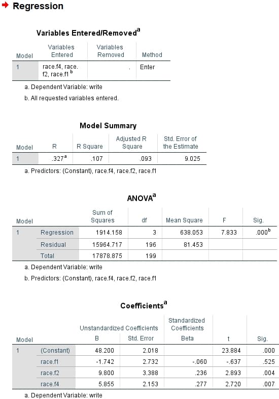
Based on this output, answer the following:

a) Write out the complete estimated regression equation.
b) Provide a precise, exam-style interpretation for the coefficient of the race.f2 variable.
c) Interpret the Adjusted R-squared value in the context of this model.
d) What do the F-statistic and its associated p-value (Sig.) tell you about the overall model? State your conclusion clearly.

Question 3: Master Derivation Challenge (15 minutes)

This question requires you to reverse-engineer a complex R output. It is a direct test of your ability to navigate interconnected formulas under pressure.

Question 4: Rapid-Fire Concepts (10 minutes)

Answer the following conceptual questions concisely.

a) You are comparing two models. Model A has an R-squared of 0.85 and an Adjusted R-squared of 0.72. Model B has an R-squared of 0.83 and an Adjusted R-squared of 0.81. Which model is likely better, and why?

b) In a Residuals vs. Fitted plot, you observe that the vertical spread of the residuals forms a distinct cone shape (it widens as fitted values increase). What assumption is violated, and what is the technical term for this problem?

c) The Variance Inflation Factor (VIF) for a predictor in your model is 30. What problem does this indicate, and what is the primary consequence for your model's coefficient estimates?

d) A fellow student interprets a slope coefficient of 50 as: "A one-unit increase in X causes the predicted Y to increase by 50." Correct this statement and explain the trap they fell into.

Answer Key

Check your answers against the detailed solutions below. Pay close attention not just to the numerical result, but also to the precision of the interpretations.

Solution to Question 1

a) Completed ANOVA Table:

Calculations:

• DF (Total): $n-1=16-1=15$
• DF (Regression): For simple linear regression, $k=1$. So, DF = 1.
• DF (Error): $d{f}_{Total}-d{f}_{Reg}=15-1=14$.
• SS (Regression): Since MSR = SSR / $d{f}_{Reg}$, then SSR = MSR $\times$ $d{f}_{Reg}$ = 309.9 $\times$ 1 = 309.9.
• SS (Error): SSE = SST - SSR = 995.95 - 309.9 = 686.05.
• MS (Error): MSE = SSE / $d{f}_{Error}$ = 686.05 / 14 = 49.003 (rounded to 49.00).
• F-statistic: F = MSR / MSE = 309.9 / 49.003 = 6.324 (or 309.9/49.0=6.32). Your value might differ slightly based on rounding, 6.368 is derived from the image's request for one decimal on SS/MS. Using 686.1 for SSE and 49.0 for MSE gives F=6.324.

b) Hypotheses:
* $H_0:{\beta }_1=0$. The model is not statistically significant; the predictor has no linear relationship with the response.
* $H_1:{\beta }_1\ne 0$. The model is statistically significant; a linear relationship exists.

c) Conclusion: The calculated F-statistic ($\approx 6.32$) is greater than the critical F-value of 4.60. Therefore, we reject the null hypothesis. There is sufficient evidence at the $\alpha =0.05$ level to conclude that the regression model is statistically significant.

Solution to Question 2

a) Estimated Regression Equation:
$\widehat{\text{write}}=48.200-1.742(\text{race.f1})+9.800(\text{race.f2})+5.855(\text{race.f4})$

b) Interpretation of race.f2 coefficient: Holding all other variables constant, the predicted 'write' score for a student in the race.f2 group is, on average, 9.800 points higher than for a student in the baseline reference group.

c) Interpretation of Adjusted R-squared: After accounting for the number of predictors in the model, approximately 9.3% of the variability in the 'write' score is explained by the race variables.

d) Conclusion for Overall F-test: The F-statistic is 7.833 with a p-value (Sig.) of .000. Since the p-value is less than 0.05, we reject the null hypothesis that all slope coefficients are zero. We conclude that the model as a whole is statistically significant, meaning at least one race category is a significant predictor of the 'write' score.

Solution to Question 3

Here are the derivations for the 10 missing values from the R output:

1. {1?} (t value for OPRC): $t=\frac{\text{Estimate}}{\text{Std. Error}}=\frac{4589.7}{309.0}=14.853$
2. {2?} (Residual df): $d{f}_{Res}=n-k-1=43-2-1=40$. (n=43 years, k=2 predictors)
3. {3?} (p-value for OPRC): The t-value of 14.853 on 40 df is extremely large. The p-value will be very small, much less than 0.001. So, < 2.2e-16 or simply < 0.001.
4. {4?} (Significance code for OPRC): Since the p-value is < 0.001, the significance code is ***.
5. {5?} (Mean Sq for Residuals): From the ANOVA table, MS(Res) = SS(Res) / Df(Res) = $\frac{3.9586\times 10^9}{40}=9.8965\times 10^7$. (This is also the square of the Residual standard error: $9948^2\approx 9.896\times 10^7$).
6. {6?} (F value for OPRC): F = MS(OPRC) / MS(Res) = $\frac{2.1836\times 10^{10}}{9.8965\times 10^7}=220.644$.
7. {7?} (Multiple R-squared): $R^2=\frac{\text{SSR}}{\text{SST}}=\frac{\text{SSR}}{\text{SSR+SSE}}$.
   • SSR = SS(APMAM) + SS(OPRC) = $1.5567\times 10^9+2.1836\times 10^{10}=2.33927\times 10^{10}$.
   • SST = SSR + SSE = $2.33927\times 10^{10}+3.9586\times 10^9=2.73513\times 10^{10}$.
   • $R^2=\frac{2.33927\times 10^{10}}{2.73513\times 10^{10}}=0.8552$.
8. {8?} (F-statistic for overall model): $F=\frac{\text{MSR}}{\text{MSE}}$
   • MSR = SSR / $d{f}_{Reg}$ = $(2.33927\times 10^{10})/2=1.1696\times 10^{10}$.
   • MSE = $9.8965\times 10^7$.
   • F = $\frac{1.1696\times 10^{10}}{9.8965\times 10^7}=118.18$.
9. {9?} (Numerator DF for F-statistic): This is $k$, the number of predictors. So, 2.
10. {10?} (Denominator DF for F-statistic): This is the residual degrees of freedom, which we found in {2?}. So, 40.

Solution to Question 4

a) Model B is preferable. While Model A has a slightly higher R-squared, its Adjusted R-squared is much lower. Adjusted R-squared penalizes the inclusion of unnecessary predictors. The higher Adjusted R-squared of Model B (0.81 vs 0.72) indicates it has better explanatory power after accounting for model complexity.

b) The assumption of homoscedasticity (constant variance of residuals) is violated. The technical term for this problem is heteroscedasticity.

c) A VIF of 30 indicates a severe multicollinearity problem. The primary consequence is that the standard errors of the coefficient estimates become highly inflated. This makes the estimates unstable and unreliable, and it becomes difficult to determine the statistical significance of individual predictors.

d) The student fell into the correlation is not causation trap. The corrected statement should be: "Holding other variables constant, a one-unit increase in X is associated with a predicted increase of 50 units in Y, on average." Regression describes relationships in the data; it does not prove that a change in one variable causes a change in another.

Conclusion

Congratulations on completing the mock exam. You have now faced the types of questions, calculations, and interpretations that are central to a practical regression exam. You have practiced deriving missing values, interpreting complex outputs, and articulating your reasoning with the precision your professor requires.

This exercise, combined with the comprehensive review from our previous sessions, puts you in a strong position for your exam tomorrow. Review your answers and the solutions carefully to solidify any final points of confusion. You have put in the focused work and are well-prepared. Walk into your exam with confidence. You've got this.