Understanding ANOVA: Deconstructing the Sums of Squares

Welcome to our third lesson. In our previous session, we tackled the critical difference between R-squared and Adjusted R-squared, establishing why the latter is essential for comparing models. In that discussion, we repeatedly encountered two key terms from the R-squared formula, $R^{2} = 1 - \frac{S S E}{S S T}$ : the Total Sum of Squares (SST) and the Error Sum of Squares (SSE).

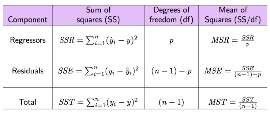
Today, we will formally deconstruct these concepts. You'll learn exactly what SST, SSE, and a third component, the Regression Sum of Squares (SSR), represent. Understanding this fundamental decomposition of variance is a non-negotiable skill for your exam. It's the bedrock of the ANOVA table and the key to both interpreting model significance and reverse-engineering missing values from partial outputs.

The Core Idea: Decomposing Variability

At its heart, regression analysis is about explaining variation. The values of your response variable, $y$ , are not all the same; they vary. The goal of a regression model is to explain as much of that variation as possible using your predictor variables.

The total variation in your response variable can be broken down into two pieces:

Explained Variation: The portion of the total variation that your regression model successfully accounts for.
Unexplained Variation: The portion that is left over, which we call error or residual.

This is the central principle of the ANOVA (Analysis of Variance) approach in regression. The "Sum of Squares" values are simply how we quantify these different buckets of variation.

This diagram illustrates the core concept: The Total Sum of Squares (SST), representing the total variation in the data, is partitioned into the Model Sum of Squares (SSM, also known as SSR) and the Error Sum of Squares (SSE).

Let's define each component precisely.

The Three Sums of Squares

The following article provides clear, concise definitions for SST, SSR, and SSE. We will walk through each one.

Sum of Squares: SST, SSR, SSE – 365 Data Science

This article from 365 Data Science defines the three core components of the Sum of Squares.

Read the section "SST, SSR, SSE: Definition and Formulas". As you read, focus on connecting each term to the concepts of total, explained, and unexplained variation. Pay close attention to the variables used in each formula (e.g., y_i, \bar{y}, \hat{y}_i).

Let's break down what you just read.

1. Total Sum of Squares (SST)

What it is: SST measures the total variability in the observed response variable, $y$ . It calculates the sum of the squared differences between each individual data point ( $y_{i}$ ) and the overall mean of the response variable ( $y ˉ$ ).
Formula: $S S T = \sum_{i = 1}^{n} (y_{i} - y ˉ)^{2}$
Exam Interpretation: Think of SST as the baseline. It's the total amount of variation in your dependent variable that you are trying to explain with your model. If you had no regression model at all, your best single-number guess for any $y_{i}$ would be $y ˉ$ , and SST represents the total squared error of that naive "mean model".

2. Regression Sum of Squares (SSR)

What it is: SSR measures the explained variation. It's the amount of variation in the response variable that is accounted for by your regression model. It calculates the sum of the squared differences between the predicted values ( $y^_{i}$ ) and the overall mean of the response ( $y ˉ$ ).
Formula: $S S R = \sum_{i = 1}^{n} (y^_{i} - y ˉ)^{2}$
Exam Interpretation: A larger SSR indicates that your model's predictions are, on average, a significant improvement over just guessing the mean. This is the "good" part of the variation—the part your model captured.

3. Error Sum of Squares (SSE)

What it is: SSE measures the unexplained variation. Also known as the Residual Sum of Squares (RSS), it's the variation that remains after accounting for your model. It is the sum of the squared differences between the observed values ( $y_{i}$ ) and the predicted values ( $y^_{i}$ ), which is simply the sum of the squared residuals.
Formula: $S S E = \sum_{i = 1}^{n} (y_{i} - y^_{i})^{2} = \sum_{i = 1}^{n} e_{i}^{2}$
Exam Interpretation: This is the quantity that Ordinary Least Squares (OLS) regression is designed to minimize. A smaller SSE means the data points are closer to the regression line, indicating a better model fit.

For a quick video recap of these definitions and the potential confusion around acronyms, watch this short clip.

Decomposition of Variability: Sum of Squares | Statistics Tutorial

This video from 365 Data Science provides a clear, visual summary of the three Sum of Squares components.

Watch from the beginning up to the summary of terms. The speaker does an excellent job of defining each term and, importantly, warns about the different notations you might see on an exam (e.g., RSS for SSE). Being aware of this is crucial to avoid misinterpreting a question.

The Fundamental Relationship: The Key to Your Exam

As both resources highlight, the three Sums of Squares are linked by one simple, powerful equation. This is the most important takeaway for your practical exam.

S S T = S S R + S S E

Total Variation = Explained Variation + Unexplained Variation

This equation is your secret weapon for reverse-engineering ANOVA tables. An exam question will almost certainly give you a partial table and expect you to fill in the blanks. With this formula, if you know any two of the Sum of Squares values, you can instantly calculate the third.

A Gentle Guide to Sum of Squares: SST, SSR, SSE

This article from Statology states the fundamental relationship very clearly.

Read the first few paragraphs of the article, ending just before the "SSR, SST & R-Squared" section. Focus on this key sentence: "The following relationship exists...". This is the core principle you will use for derivations.

Practice Drill

You are given the following output from a regression analysis of housing prices.

The total variation (SST) in house prices for the dataset is 1,250 (in millions of dollars squared).
The sum of squared residuals (SSE) from your model is 250 (in millions of dollars squared).

Your Tasks:

Calculate the Regression Sum of Squares (SSR).
In one sentence, explain what this SSR value represents in the context of the housing price model.
Calculate the R-squared of this model.

Solution

Calculate SSR:
- We use the formula: $S S T = S S R + S S E$
- Rearranging for SSR: $S S R = S S T - S S E$
- $S S R = 1250 - 250 = 1000$
Interpretation:
- The SSR of 1,000 (in millions of dollars squared) represents the portion of the total variation in housing prices that is explained by the predictor variables in our regression model.
Calculate R-squared:
- The formula for R-squared is $R^{2} = \frac{S S R}{S S T}$
- $R^{2} = \frac{1000}{1250} = 0.80$
- This means our model explains 80% of the variability in housing prices.

Conclusion

You have now deconstructed the first, and most important, column of the ANOVA table: the Sum of Squares. This is a major step toward mastering exam outputs.

Key Takeaways for Your Exam:

SST (Total): The total variation in the dependent variable around its mean. This is your starting point.
SSR (Regression): The variation explained by your model. This is your model's contribution.
SSE (Error): The variation unexplained by your model. This is the leftover residual error.
The Golden Rule: $S S T = S S R + S S E$ . This is the key to deriving missing values.

In the next lesson, we will build upon this foundation. We will add the "Degrees of Freedom" (df) column to our understanding, which will allow us to calculate "Mean Squares" (MSR and MSE). This will lead us directly to calculating and interpreting the F-statistic, which tests the overall significance of your entire model.

Recommended resources