Put-Call Parity and Option Pricing

Introduction

In our last lesson, we focused on calculating the profit and loss for individual call and put options. We now have a solid grasp of how the value of a single option position behaves at expiration. Today, we'll explore a crucial relationship that connects these seemingly separate instruments: put-call parity.

This lesson introduces a fundamental principle based on the concept of no-arbitrage, a cornerstone of financial engineering. You will learn how to apply the put-call parity formula, which links the prices of a European call option, a European put option, the underlying stock, and a risk-free bond. The core of today's work will be numerical application—using this elegant equation to determine what the price of an option should be, given the prices of the others. This directly addresses the learning outcome and will provide you with a powerful tool for your CB1 exam toolkit.

1. The Foundation: No-Arbitrage and Equivalent Portfolios

At the heart of put-call parity is the law of one price: two portfolios that guarantee the exact same payoff in the future, regardless of what happens, must have the same price today. If they don't, a risk-free profit, known as arbitrage, would be possible.

To understand this, we'll construct two different portfolios whose payoffs at expiration are identical.

Portfolio A: Fiduciary Call. This consists of one European call option and a zero-coupon bond that matures at the option's expiration with a face value equal to the strike price, $K$ .
Portfolio B: Protective Put. This consists of one European put option and one share of the underlying stock.

Let's watch a video that introduces these two strategies and visually demonstrates why their payoffs are identical.

CFA Level I Derivatives - Put-Call Parity

The video "CFA Level I Derivatives - Put-Call Parity" from PrepNuggets provides an excellent, step-by-step derivation of the parity relationship.

Please watch the following two segments: First, focus on the protective put from the introduction. Note how combining a long stock and a long put creates a payoff with limited downside. Next, watch the explanation of the fiduciary call from this section. Observe how combining a long call with a risk-free bond results in the very same payoff profile as the protective put.

As the video shows, both portfolios have a final value of $K$ if the stock price at expiration ( $S_{T}$ ) is below the strike price, and a value of $S_{T}$ if the stock price is above the strike price. Since their future payoffs are identical, their costs today must be equal to prevent arbitrage.

2. The Put-Call Parity Formula

By equating the initial costs of our two portfolios, we arrive at the put-call parity formula. Let's denote the initial prices as:

$c_{0}$ : Call premium
$p_{0}$ : Put premium
$S_{0}$ : Stock price
$K$ : Strike price
$P V (K)$ : The present value of the strike price, which is the price of the zero-coupon bond.

The cost of the fiduciary call is $c_{0} + P V (K)$ . The cost of the protective put is $p_{0} + S_{0}$ . Equating these gives the relationship:

c_{0} + P V (K) = p_{0} + S_{0}

Typically, the present value is calculated using the risk-free rate, $r$ , and the time to expiration, $T$ . For continuous compounding, $P V (K) = K e^{- r T}$ . For discrete compounding, $P V (K) = K (1 + r)^{- T}$ . For the CB1 exam, you should be comfortable with both, but we'll often use the discrete version for simplicity unless specified.

The AnalystPrep article below provides a clear, written summary of this derivation, including a helpful table that confirms the identical payoffs.

Put-Call Parity Explained | CFA Level 1

This article from AnalystPrep neatly summarises the logic we've just discussed.

Please read the first part of the article, from the beginning down to the formula. Focus on the table titled Payoff Table. This table is the formal proof that the two portfolios have identical values at expiration under all scenarios.

3. Applying the Formula: Calculating Option Prices

The primary use of put-call parity is to find the fair price of one asset when the prices of the other three are known. Let's work through an example.

Problem: A European put and call option on a non-dividend-paying stock both have a strike price of $50 and expire in 3 months (0.25 years). The underlying stock is priced at $52. The put is trading for $3.80, and the annual risk-free rate is 4.5%. What is the no-arbitrage price of the call option?

Solution:
We use the formula $c_{0} + K (1 + r)^{- T} = p_{0} + S_{0}$ and rearrange it to solve for $c_{0}$ :

c_{0} = p_{0} + S_{0} - K (1 + r)^{- T}

Plugging in the values:

$p_{0} = $3.80$
$S_{0} = $52$
$K = $50$
$r = 0.045$
$T = 0.25$

c_{0} = 3.80 + 52 - 50 (1.045)^{- 0.25}

First, calculate the present value of the strike price:

50 (1.045)^{- 0.25} \approx 50 \times 0.9890 = $49.45

Now, substitute this back into the main equation:

c_{0} = 3.80 + 52 - 49.45 = $6.35

The no-arbitrage price for the call option is $6.35. If the call were trading at any other price, a risk-free profit would be possible.

Now, let's review a similar example from the AnalystPrep article.

Put-Call Parity Explained | CFA Level 1

The article we looked at earlier provides another clear, worked example.

Read the section titled Example. This walks through the exact calculation we just performed.

4. What if Parity Fails? Arbitrage in Action

If the put-call parity equation does not hold, an arbitrage opportunity exists. Your strategy is simple: sell the overpriced portfolio and buy the underpriced portfolio. This will generate a positive cash flow today, and because the portfolios have identical payoffs at expiration, your future cash flows will net to zero. You are left with a risk-free profit.

Let's watch a video that demonstrates this with a clear numerical example in Excel.

Put-Call Parity in Options Trading Explained Using Excel

The video "Put-Call Parity in Options Trading Explained Using Excel" by Ryan O'Connell is excellent for understanding arbitrage.

Watch from the beginning to see how the two portfolios are valued. Then, pay close attention to the arbitrage explanation starting at this timestamp. The presenter shows that if the call is underpriced, Portfolio A (fiduciary call) is cheaper than Portfolio B (protective put). The strategy is to buy the cheap one (Portfolio A) and sell the expensive one (Portfolio B). Finally, watch the section from this proof which demonstrates why the arbitrage is risk-free by showing the identical payoffs at expiration.

The key takeaway is that the market's collective search for such arbitrage opportunities is what enforces put-call parity. In an efficient market, these mispricings are quickly identified and eliminated.

5. Synthetic Positions

A final powerful insight from put-call parity is the concept of synthetic positions. By rearranging the formula, we can show that any one of the four assets can be replicated by a combination of the other three.

For example, rearranging for the stock gives:

S_{0} = c_{0} - p_{0} + K (1 + r)^{- T}

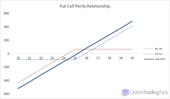
This means you can create a "synthetic stock" by buying a call, selling a put, and investing the present value of the strike price in a risk-free bond. The payoff profile of this combination will exactly match that of holding the stock itself.

The diagram below shows a simplified version of this, where combining a long call and a short put creates a payoff profile that looks very much like holding the underlying stock.

This graph illustrates how the payoff of a long call (blue dotted line) combined with the payoff of a short put (red dotted line) results in a linear payoff profile similar to that of a long stock position (solid blue line). This visualizes the concept of a "synthetic forward," a core idea in put-call parity.

Conclusion

Today we've uncovered one of the most elegant and practical relationships in finance. Put-call parity is more than just a formula; it's a reflection of the no-arbitrage condition that underpins modern financial markets.

Key Takeaways:

Put-call parity states that the price of a protective put ( $p_{0} + S_{0}$ ) must equal the price of a fiduciary call ( $c_{0} + P V (K)$ ), assuming European options and no dividends.
The relationship is enforced by arbitrageurs who would buy the cheaper portfolio and sell the more expensive one if a mispricing occurred.
The formula can be rearranged to solve for the fair price of any one of the four components (call, put, stock, bond) if the other three are known.
This relationship only holds for European options, which can only be exercised at expiration.

In our next lesson, we will shift our focus to another major class of derivatives: swaps. You will learn how interest rate swaps and currency swaps are structured and how to calculate the cash flows exchanged between the parties involved.

Recommended resources