Hedging with Derivatives

1. Hedging Interest Rate Risk

Interest rate risk is the potential for losses arising from changes in interest rates. For a company with a floating-rate loan, the risk is that interest rates will rise, increasing their interest payments. Conversely, for an investor holding floating-rate assets, the risk is that rates will fall, reducing their income. We will focus on the borrower's perspective.

Hedging a Single Future Period: Forward Rate Agreements (FRAs)

When a company needs to borrow at a floating rate for a specific, single period in the future, it can lock in an interest rate today using a Forward Rate Agreement (FRA). An FRA is an over-the-counter contract between two parties to agree on an interest rate to be applied to a notional principal amount for a future period.

The video below provides an excellent explanation of what an FRA is and walks through a complete numerical example. This will show you exactly how an FRA is selected and how it achieves a fixed effective interest rate for the borrower.

To summarise the logic from the video:

1. The Agreement: The company agrees on a forward rate (e.g., 3.85%) with a bank.
2. The Outcome: At the start of the loan period, the actual market rate (LIBOR/SOFR) turns out to be higher (e.g., 4.0%). The company borrows at this higher rate from the market.
3. The Compensation: Because the market rate is higher than the agreed FRA rate, the bank compensates the company for the difference (4.0% - 3.85% = 0.15%).
4. The Result: The compensation payment effectively reduces the company's total interest cost back down. The final effective interest rate paid by the company is fixed, regardless of the market rate's movement.

Hedging a Long-Term Floating Rate Loan: Interest Rate Swaps

While FRAs are for single periods, interest rate swaps are the primary tool for hedging a floating-rate exposure that spans multiple years. The most common application is to convert a floating-rate loan into a synthetic fixed-rate loan.

Let's revisit the swap structure, which we first saw in the context of currency risk. The logic here is similar, but instead of exchanging different currencies, both legs of the swap are in the same currency, just calculated on different interest rate bases (fixed vs. floating).

The diagram below illustrates how a company (Fund A) with a floating-rate loan (LIBOR + 2%) can use a swap to fix its interest cost.

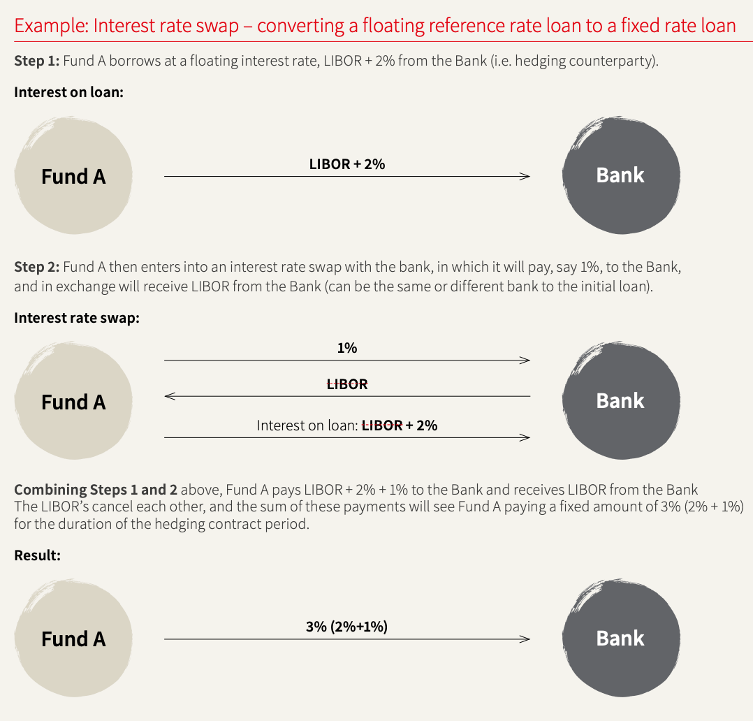
Let's break down the mechanics shown in the diagram:

• Step 1: The Loan. Fund A has a loan where it pays a variable interest rate of LIBOR + 2% to a bank. This exposes the fund to the risk of LIBOR increasing.
• Step 2: The Swap. Fund A enters into an interest rate swap with a counterparty (which could be the same bank or a different one). In this swap, Fund A agrees to:
  • Pay a fixed rate of 1%.
  • Receive a floating rate of LIBOR.
• Step 3: The Net Effect. We can now combine the cash flows:
  • Interest paid on loan: -(LIBOR + 2%)
  • Interest paid on swap: -1%
  • Interest received on swap: +LIBOR
  • Total Interest Cost: -(LIBOR + 2%) - 1% + LIBOR = -3%

The floating LIBOR payments cancel each other out. Fund A has successfully transformed its volatile floating-rate payment into a stable, predictable fixed payment of 3%.

For a more formal definition and a detailed cash flow table that demonstrates this effect over several periods with changing rates, please review the following document.

2. Hedging Equity Price Risk

For an investor holding a diversified portfolio of stocks, the primary risk is not that one particular company will do poorly (this is unsystematic risk, which can be diversified away), but that the entire market will decline. This is systematic risk, and it is measured by the portfolio's beta ($\beta$). A beta of 1.0 means the portfolio tends to move in line with the market. A beta of 1.5 means it's 50% more volatile than the market.

The Solution: Hedging with Equity Index Futures

To hedge against a fall in the overall market, a portfolio manager can sell equity index futures. A futures contract is a standardized, exchange-traded agreement to buy or sell an asset at a predetermined price on a future date.

By selling (or "shorting") index futures, the manager creates a position that will profit if the market falls. This profit is designed to offset the loss on their actual stock portfolio. The key question is: how many futures contracts should be sold to achieve the hedge? The answer is given by the beta-adjusted hedge ratio.

The following article explains this concept clearly and provides the necessary formula and a worked example.

The core formula from the article to calculate the number of contracts (N) needed to adjust a portfolio's beta is:

Where:

• ${\beta }_{\text{target}}$ is the desired portfolio beta after hedging (e.g., 0 for a full hedge).
• ${\beta }_{\text{portfolio}}$ is the current beta of the portfolio.
• $V_P$ is the total value of the portfolio.
• $V_F$ is the notional value of one futures contract (Futures Price × Multiplier).

A negative result for $N$ indicates you need to sell futures contracts to reduce the beta.

A Deeper Look: Static vs. Dynamic Hedging

A key challenge in hedging is that a portfolio's beta (or an option's delta) is not constant. It changes as market conditions and time evolve. This leads to a crucial distinction between two approaches to hedging. This may seem advanced, but the core idea is highly relevant for understanding the practicalities of risk management.

As a statistician, you can think of beta as a sensitivity coefficient in a regression of portfolio returns on market returns. Since this coefficient is not stable over time, a hedge based on today's beta might not be perfect tomorrow.

The following video introduces this idea using the concept of Delta from options pricing. Delta is analogous to beta; it measures an option's price sensitivity to changes in the underlying stock's price. The principles of hedging sensitivity are the same.

• Static Hedging: This is a "set it and forget it" approach. You calculate the hedge ratio once and put the position on, leaving it until the end of the hedging period. It's simple and low-cost, but the hedge can become imperfect as the portfolio's beta drifts.
• Dynamic Hedging: This involves continuously monitoring the portfolio's beta and adjusting the number of futures contracts to keep the portfolio perfectly hedged (or at its target beta). This is more precise but incurs higher transaction costs.

For the purposes of the CB1 exam, understanding the static hedge calculation is sufficient. However, knowing that dynamic hedging exists provides a more complete and realistic picture of institutional risk management.

Conclusion

This lesson concludes our exploration of derivatives by demonstrating their use as powerful hedging instruments. You have seen how different risks call for different tools, and how a numerical approach is essential to implementing these strategies correctly.

Key Takeaways:

• Forward Rate Agreements (FRAs) are used to lock in an interest rate for a single, future borrowing or lending period.
• Interest Rate Swaps (IRS) are used to hedge long-term floating-rate exposures, most commonly to convert a floating-rate loan into a synthetic fixed-rate loan.
• Equity Index Futures are used to hedge the systematic risk (market risk) of a diversified equity portfolio. The number of contracts needed is determined by the portfolio's beta.
• Hedging is not a one-time event; dynamic hedging involves adjusting the hedge as risk parameters change over time.

This discussion of beta serves as a perfect bridge to our next module, "Cost of Capital and Capital Structure." In the very next lesson, we will see how beta is not just a measure of risk to be hedged, but also a crucial input for calculating the expected return on an investment through the Capital Asset Pricing Model (CAPM).