Parallel Hash Join Optimization

A Quick Review: The Single-Node Hash Join

Before we parallelize the algorithm, let's briefly recall how a basic hash join works on a single machine. If you need a more detailed refresher, the previous module on Query Execution covered this in depth.

The algorithm has two main phases:

1. Build Phase: Scan the smaller (outer) relation, and build an in-memory hash table using the join key. For example, in R JOIN S, if R is smaller, we'd build a hash table on R.
2. Probe Phase: Scan the larger (inner) relation. For each tuple, hash its join key and probe the hash table to find matching tuples from the build relation.

This is highly efficient when the hash table for the outer relation fits in memory. But what if the data is distributed across dozens or hundreds of nodes in a shared-nothing cluster? Let's find out.

The Core of Parallel Hash Join: Partition and Conquer

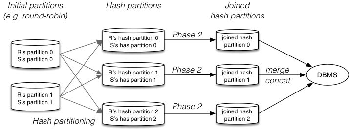
The fundamental strategy for a parallel hash join in a shared-nothing architecture is to use the Exchange (or Shuffle) operator we learned about previously. The goal is simple: ensure that all tuples from both relations that could possibly join (i.e., they have the same join key) end up on the same worker node.

This is achieved through hash partitioning on the join key:

1. Shuffle Phase: All worker nodes scan their local partitions of both relations, R and S. For each tuple, they apply a common hash function to the join attribute, h(join_key), and send the tuple to the worker node determined by the hash value (e.g., worker_id = h(join_key) % num_workers).
2. Local Join Phase: After the shuffle is complete, every worker node i holds a partition of R (let's call it Ri) and a partition of S (Si). Crucially, all tuples in Ri and Si that can join are guaranteed to be on the same node. Each worker can then perform a standard single-node hash join on its local Ri and Si partitions, completely in parallel with all other workers.

This "partition-first" or "shuffle-then-join" approach is a classic parallel database algorithm.

While this is the classic model, modern systems have evolved different architectures to implement this idea. Let's look at two prominent designs.

Architecture 1: The "No-Partition" Shared Hash Table

One popular and surprisingly effective design, used by systems like PostgreSQL, is to have all workers collaborate on building a single, large hash table in shared memory.

As you read, the key phases of this design are:

1. Shared Build: All worker processes scan the build relation in parallel and concurrently insert tuples into one giant, shared hash table. This requires thread-safe data structures and synchronization (latches) to manage concurrent writes.
2. Synchronization Barrier: A critical step. All workers must wait until every worker has finished scanning the build relation. This ensures the shared hash table is complete before anyone starts probing it.
3. Shared Probe: After the barrier, all workers scan their partitions of the probe relation in parallel and perform lookups (probes) against the now-complete shared hash table.

This "no-partition" design is simple and avoids the overhead of physically writing out intermediate partitions to disk or memory buffers.

Architecture 2: The Radix-Partition Join

The second major design is a more explicit "partition-first" strategy, often called a Radix Join. This approach focuses on breaking down the relations into many small partitions that are optimized for cache performance.

The key idea behind Radix partitioning is a multi-pass approach to data shuffling:

1. Histogram Pass: In the first pass, workers scan the build relation and create local histograms based on a few bits of the hashed join key (the "radix"). These histograms count how many tuples fall into each radix partition.
2. Prefix Sum & Shuffle Pass: The local histograms are aggregated to compute a global prefix sum. This tells each worker the exact offset in a global buffer where it should write its tuples for each radix partition. In the second pass, workers rescan the relation, and using the pre-computed offsets, write tuples into the correct partitions without any locking. This entire process is then repeated for the probe relation.
3. Local Join Phase: Once both relations are partitioned, workers can process pairs of (R, S) radix partitions, which are now small enough to fit nicely in CPU caches, and perform the final joins.

The Elephant in the Room: Data Skew

Both parallel join strategies rely on the hash function to distribute work evenly. But what happens if the data itself is not evenly distributed?

Data skew is when certain join key values appear far more frequently than others. For example, in a customers table, the country_code 'USA' might appear millions of time, while 'LUX' appears only a few thousand.

A naive hash partition (h(key) % N) will send all tuples for 'USA' to the same worker. This worker becomes a bottleneck, overloaded with data, while other workers finish quickly and sit idle. This is called redistribution skew, and it can completely undermine the benefits of parallelism.

So, how do we handle it? The classic paper "Practical Skew Handling in Parallel Joins" by DeWitt et al. provides the foundational techniques.

A Key Technique: Virtual Processor Partitioning

Instead of creating a number of partitions equal to the number of workers (N), we create many more partitions, say 100 * N. We can think of these as "virtual" partitions or fine-grained buckets.

The process is:

1. Partition both relations R and S into a large number of virtual partitions based on the join key. A heavy-hitter key might still dominate one or more virtual partitions, but each virtual partition is now a much smaller unit of work.
2. Distribute these virtual partitions to the actual worker nodes for processing. The simplest way is round-robin, where virtual partition i is assigned to worker i % N.

Because each worker now gets a mix of many small virtual partitions, the total workload tends to average out, even in the presence of skew. The large amount of work from a "heavy" virtual partition is balanced by the small amounts of work from many "light" ones.

Interestingly, the "no-partition" shared hash table approach we discussed first has a natural advantage here. As highlighted in the Postgres blog, academic research shows that this simple algorithm is very competitive and can even outperform complex partitioning algorithms when data is skewed, precisely because all workers are contributing to all keys, so no single worker gets stuck with a "hot" key.

Conclusion

We've delved into the design of the parallel hash join, a cornerstone of modern data warehouses and analytical engines. It's a fantastic real-world application of intra-operator parallelism and the Exchange operator.

Key Takeaways:

• Parallel hash joins work by shuffling both relations on the join key, ensuring matching tuples are co-located on the same worker node for a local join.
• There are two primary architectural patterns:
  • Partition-First (e.g., Radix Join): Explicitly partition data into many small, independent chunks, then join them. This can be complex but offers good cache performance and a clear path for out-of-memory processing.
  • Shared Hash Table: Have all workers build a single, concurrent hash table. This is simpler and has proven to be very robust against data skew, a critical real-world problem.
• Data skew is a major performance killer in parallel joins. It can be handled with techniques like Virtual Processor Partitioning to achieve finer-grained load balancing.

Preview of the Next Lesson

So far, our discussions of transactions, concurrency, and recovery have been in the context of a single database instance. But what happens when a transaction needs to modify data on multiple nodes in our distributed system? How can we guarantee atomicity—that the transaction either commits everywhere or aborts everywhere—especially when nodes can fail?

In the next lesson, we will tackle this challenge head-on by examining the classic algorithm for distributed transaction coordination: the two-phase commit (2PC) protocol.