Parallelism in Shared-Nothing Systems

A Quick Recap: The Shared-Nothing World

Remember, we're operating in a shared-nothing architecture. Each node is an independent computer with its own CPU, memory, and disk, connected only by a network.

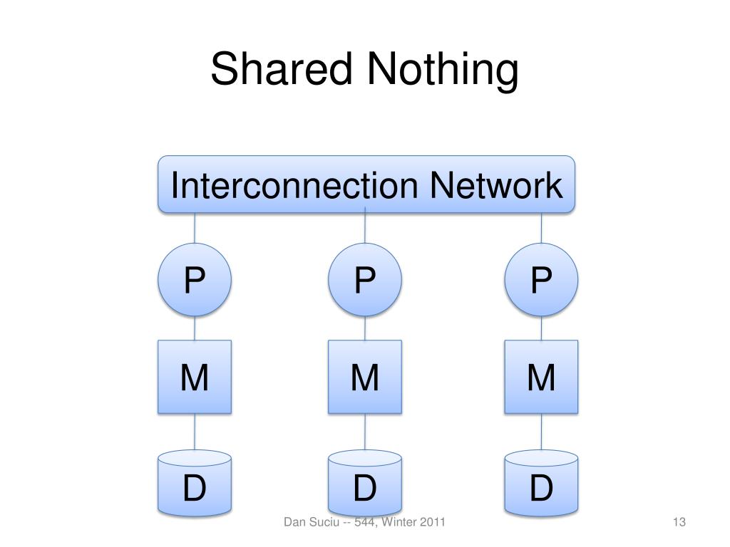
Because our data is partitioned across these nodes, we have a natural opportunity for parallelism. Instead of one machine doing all the work, we can have many machines working on their piece of the data simultaneously. This is the essence of intra-query parallelism: making a single query run faster by parallelizing its execution.

Let's dive into the two primary ways this is achieved.

Now, let's break down these concepts with more detail and examples.

1. Inter-Operator Parallelism (Pipelined Parallelism)

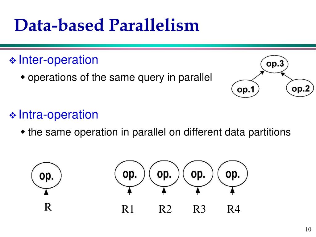
As the name suggests, inter-operator parallelism involves executing different operators within the same query plan concurrently. Think of it as a factory assembly line.

Imagine a simple query: SELECT * FROM sales WHERE amount > 1000;

A query optimizer might generate a simple plan: Scan(sales) -> Filter(amount > 1000).

With inter-operator parallelism, the Scan operator doesn't need to finish reading the entire sales table before the Filter operator can begin. As soon as Scan produces its first row (or page of rows), it can "pipe" that output directly to the Filter operator, which can then immediately evaluate the condition amount > 1000.

This creates a pipeline of operators, where data flows through the stages of the query plan. It's also known as pipelined parallelism or vertical parallelism.

The "Bubble" Problem

This pipeline approach is efficient, but it's not perfect. A pipeline is only as fast as its slowest stage. If one operator in the pipeline is very slow, or if it's a blocking operator (like Sort, which must consume all its input before it can produce any output), the downstream operators will be starved for data, sitting idle. This idle time is often called a "pipeline bubble."

Interestingly, this exact concept and terminology are central to another area of large-scale systems: training massive machine learning models.

The key takeaway is that inter-operator parallelism allows for concurrent execution of different tasks in a query, but its efficiency can be limited by dependencies and blocking operations that break the smooth flow of the pipeline.

2. Intra-Operator Parallelism (Partitioned Parallelism)

While inter-operator parallelism runs different operators at the same time, intra-operator parallelism runs multiple instances of the same operator on different subsets of data concurrently. This is where our data partitioning from the last lesson becomes critical.

This is also known as partitioned parallelism or horizontal parallelism.

Let's go back to our query: SELECT * FROM sales WHERE amount > 1000;

Assume the sales table is partitioned across 10 nodes. With intra-operator parallelism, the database can launch 10 instances of the Scan operator and 10 instances of the Filter operator. Each pair of Scan -> Filter runs on one of the 10 nodes, processing its local partition of the sales table completely in parallel.

The Exchange Operator: The Glue for Parallelism

Intra-operator parallelism is straightforward when an operation can be performed locally on each partition (like a scan or a filter). But what happens when an operator needs data from multiple partitions? For example, a JOIN between two partitioned tables, or a GROUP BY aggregation.

This is where a special operator called Exchange (or Shuffle/Repartition) comes in. The Exchange operator is responsible for moving data across the network between nodes. It's the physical implementation of data redistribution within a query plan.

As detailed in the CMU notes (LINK), the Exchange operator has three main forms:

1. Gather: Merges data from many parallel workers into a single output stream on one worker. This is used at the end of a query to collect final results.
2. Distribute: Splits the output of one worker and distributes it to many workers.
3. Repartition / Shuffle: Reorganizes data from M input workers to N output workers, typically based on a hash function on a specific key (e.g., the join key or group by key). This is the workhorse behind parallel joins and aggregations.

Combining Both Types of Parallelism

The true power of a parallel DBMS comes from combining both inter- and intra-operator parallelism in a single query plan.

Consider this query on a shared-nothing system where users and orders are partitioned by user_id across 4 nodes:

SELECT
  u.country,
  COUNT(o.order_id)
FROM users u
JOIN orders o ON u.user_id = o.user_id
WHERE u.signup_date > '2023-01-01'
GROUP BY u.country;

A parallel execution plan might look like this:

1. Intra-operator Parallelism: On each of the 4 nodes, a Scan and Filter pipeline runs on the local users partition. At the same time, a Scan runs on the local orders partition.
2. Inter-operator Parallelism: The Scan on users pipes its output directly to the Filter.
3. Intra-operator Parallelism: Since both tables are partitioned on user_id, the JOIN can be performed locally on each node in parallel. This is called a "co-located join." Each of the 4 nodes joins its local users data with its local orders data.
4. Exchange (Shuffle): The results of the local joins now need to be aggregated by country. The query engine initiates a shuffle. Each of the 4 nodes hashes the country for its intermediate results and sends the rows to the appropriate destination node. For example, all rows for 'USA' might go to Node 1, 'Canada' to Node 2, and so on.
5. Intra-operator Parallelism: Each node now has a subset of the joined data, grouped by country. It performs a partial COUNT(*) aggregation in parallel.
6. Exchange (Gather): Finally, the partial counts from each node are gathered to a single coordinator node, which sums them up to produce the final result.

This example shows how the two types of parallelism work together, with the Exchange operator orchestrating the necessary data movement between parallel stages.

Conclusion

In this lesson, we dissected the two fundamental strategies for parallel query execution that allow distributed databases to leverage the power of a shared-nothing cluster.

Key Takeaways:

• Intra-query parallelism is about speeding up a single query.
• Inter-operator (Pipelined) Parallelism executes different operators of a query plan concurrently, like an assembly line. Its main weakness is its sensitivity to slow or blocking operators.
• Intra-operator (Partitioned) Parallelism executes multiple instances of the same operator on different data partitions simultaneously. This is the key to achieving massive scalability in shared-nothing systems.
• The Exchange (or Shuffle) operator is the critical component that moves and reorganizes data between nodes, enabling complex parallel operations like joins and aggregations.

Preview of the Next Lesson

We've now covered the "what" and "how" of parallel execution conceptually. In our next lesson, we will apply these principles to a cornerstone algorithm of any parallel database: the join. We will design and analyze a parallel hash join algorithm, including data shuffling and skew handling, which is a perfect real-world application of the concepts we learned today.