Estimating Predicate Selectivity with Histograms

From Uniformity to Distribution: The Need for Histograms

As we discussed, assuming that all values in a column are equally common is a convenient but often incorrect simplification. If we have a status column where 'active' accounts for 99% of rows and 'archived' for 1%, using the formula sel = 1 / V(A,R) for a query WHERE status = 'archived' would be off by orders of magnitude.

Storing the exact frequency of every single value would provide perfect estimates, but this is impractical. For a column with millions of distinct values, the statistics would be as large as the column itself!

Histograms offer a practical middle ground. They are data structures that approximate the distribution of values in a column by grouping them into a fixed number of buckets. This provides a compressed summary that is much more accurate than a simple average but far smaller than storing exact counts.

The Two Flavors: Equi-Width vs. Equi-Depth

As the video introduced, there are two primary strategies for creating histogram buckets. Their structures are a direct result of how they handle the trade-off between implementation simplicity and accuracy in the face of data skew.

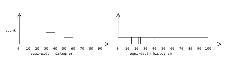
Let's formalize these concepts.

1. Equi-Width Histograms

In an equi-width histogram, the entire range of values for a column (from min_val to max_val) is divided into a set number of buckets, each covering an identical width or range of values.

• Structure: Each bucket stores a count of the number of tuples whose values fall within its specific range.
• Pros: Very simple to construct and maintain. The bucket for any given value can be found with a quick arithmetic calculation.
• Cons: Ineffective for skewed data. If a few values are extremely common, they will be grouped into a single bucket with a very high count, while many other buckets might be sparse or empty. Information about the distribution within that high-density bucket is lost.

2. Equi-Depth Histograms (or Equi-Height)

In an equi-depth histogram, the goal is for every bucket to hold approximately the same number of tuples.

• Structure: The bucket boundaries are adjusted so that each bucket represents a different width in the value range. Dense regions of data will have narrow buckets, while sparse regions will have wide buckets.
• Pros: Adapts gracefully to data skew. It provides more detailed information (i.e., more buckets) for the most frequent value ranges, which is precisely where better estimates are needed. This generally leads to better accuracy.
• Cons: More complex to construct, as it requires sorting the column values (or a sample of them) to determine the bucket boundaries.

Because of their superior accuracy on skewed data, equi-depth histograms are more commonly used in modern database systems.

Using Histograms to Estimate Selectivity

Now for the core of the lesson: how does the optimizer use these structures to calculate selectivity? The general principle is to locate the relevant bucket(s) and then assume a uniform distribution within that bucket.

A. Estimating for Equality Predicates (WHERE col = value)

1. The optimizer identifies which bucket the value falls into.
2. It retrieves the total count of items in that bucket.
3. It assumes the items are uniformly distributed within the bucket's value range.
4. The estimated count for the specific value is calculated as (count in bucket) / (number of distinct values in bucket). If the number of distinct values is not stored, it's often approximated from the range.
5. Selectivity = (Estimated Count) / (Total Tuples in Table)

B. Estimating for Range Predicates (WHERE col > value)

1. The optimizer identifies the bucket where the value lies.
2. Partial Bucket Calculation: For this bucket, it calculates the fraction of the range that satisfies the predicate. For example, if the bucket covers values [30, 40] and the predicate is > 35, it assumes (40 - 35) / (40 - 30) = 50% of the rows in that bucket match. This is a form of linear interpolation.
3. Full Bucket Calculation: It adds the full counts of all buckets that are completely within the range (i.e., all buckets whose lower bound is greater than value).
4. The total estimated count is the sum from the partial bucket and all full buckets.
5. Selectivity = (Total Estimated Count) / (Total Tuples in Table)

A Practical Look: Histograms in PostgreSQL

To ground this theory in a real system, let's look at how a popular open-source database like PostgreSQL handles this. Real-world implementations often add a layer of sophistication. For extremely skewed data, even an equi-depth histogram might not be ideal. A few values can be so common that they deserve special treatment.

PostgreSQL combines two techniques:

1. Most Common Values (MCV) List: It stores a separate list of the most frequent values and their exact frequencies.
2. Histogram: It then builds a histogram on the remaining values that are not in the MCV list.

When estimating selectivity, the optimizer first checks if the value is in the MCV list. If so, it uses the exact frequency. If not, it uses the histogram as described above.

This hybrid approach allows the optimizer to be highly accurate for the most common values (which often have the biggest impact on query cost) while still having a good general model for the rest of the data distribution.

Conclusion

You have now explored the primary mechanism that database optimizers use to overcome the flawed assumption of uniform data distribution. Understanding histograms is key to appreciating how a database can intelligently estimate the costs of its operations.

Key Takeaways:

• Histograms approximate the data distribution in a column by grouping values into buckets.
• Equi-width histograms have buckets of equal value range, making them simple but less effective for skewed data.
• Equi-depth histograms have buckets with roughly equal numbers of tuples, making them better at adapting to data skew and generally more accurate.
• Selectivity is estimated by locating the relevant bucket(s) and assuming uniform distribution within a bucket, using linear interpolation for partial buckets.
• Real systems like PostgreSQL often use a hybrid approach, combining Most Common Values (MCV) lists for very frequent items with histograms for the rest of the data.

Preview of the Next Lesson

So far, we have focused on estimating the cardinality of SELECT operations on a single table. The next major challenge is estimating the result size of a JOIN. In our next lesson, we will learn how to estimate the cardinality of join operations using foreign key statistics, which is another critical input for choosing the most efficient join order and algorithm.