Cardinality Estimation for Foreign Key Joins

The Amplifying Effect of Bad Join Estimates

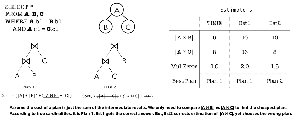
Before we dive into formulas, let's build some intuition for why join cardinality estimation is so critical. The output of one join is the input to the next operator. If the optimizer thinks a join will produce 1,000 rows but it actually produces 1 million, the cost calculations for every subsequent step in the plan will be drastically wrong.

The General Case and Its Flaws

For a general equijoin between two tables R and S on columns A and B (R.A = S.B), a simple approach, assuming uniform data distribution, is:

Here, V(A, R) is the number of distinct values in column A of table R. This formula essentially calculates the probability of a value from R matching a value from S and multiplies it by the size of the Cartesian product.

However, like the simple selectivity estimates we saw in the last lesson, this formula relies on assumptions that are often violated:

• Uniform Distribution: It assumes all values are equally frequent.
• Value Inclusion: It assumes the set of values in R.A and S.B are roughly the same.

What if one set of keys is a strict subset of the other? This happens constantly in normalized database schemas. This is where foreign keys provide a powerful hint to the optimizer.

The Foreign Key Shortcut: A Powerful Simplification

A foreign key constraint creates a "one-to-many" or "parent-child" relationship. The constraint guarantees that every value in the foreign key column of the "child" table must exist in the primary key column of the "parent" table.

This guarantee is a gold mine for the optimizer. When joining a child table to its parent on this key, every single row from the child table will find exactly one matching row in the parent table.

This leads to a beautifully simple estimation rule.

As the slides explain, if you are joining R (parent) and S (child) on the foreign key, the cardinality of the result is simply the cardinality of the child table, |S|.

For example, consider a query joining Orders and Customers:

SELECT Orders.OrderID, Customers.CustomerName
FROM Orders
JOIN Customers ON Orders.CustomerID = Customers.CustomerID;

Since Orders.CustomerID is a foreign key referencing Customers.CustomerID, every order has exactly one customer. Therefore, the number of rows in the join result will be exactly the number of rows in the Orders table. The optimizer can use this fact to get a perfect cardinality estimate for this join without needing complex histograms.

A Practical Deep Dive: When "Smarter" is Dumber

Your background and goals point to an interest in how systems work under the hood, including their non-obvious failure modes. The foreign key shortcut is powerful, but what happens if an engineer, thinking "more stats are always better," decides to create detailed histograms on both the primary and foreign key columns?

This next resource—a classic blog post from an Oracle performance expert—explores exactly this scenario. It's a perfect example of how a deep understanding of internals can explain seemingly bizarre optimizer behavior.

This "Mystery of Halving" is a profound lesson in systems design. The complex, histogram-aware join algorithm had an implementation detail that caused it to fail in this common scenario. In contrast, the simpler "standard formula," when applied to a parent-child join, simplifies perfectly:

num_rows(parent) * num_rows(child) / max(num_distinct(parent), num_distinct(child))

Since num_distinct(parent) will be equal to num_rows(parent) (for a primary key) and num_distinct(child) is less than or equal to num_distinct(parent), the max term is num_distinct(parent). The formula becomes:

num_rows(parent) * num_rows(child) / num_distinct(parent)

And since num_rows(parent) = num_distinct(parent) for a primary key, this cancels out, leaving:

num_rows(child)

The simple model, leveraging the structural knowledge of the primary key, arrives at the perfect answer. This shows that the optimizer's best strategy is often to trust the structural constraint (FOREIGN KEY) more than a complex statistical model that might have corner-case flaws.

Conclusion

You've now learned the most important technique for estimating the size of joins. While general-purpose histogram-based methods exist, leveraging structural database constraints like foreign keys provides a shortcut that is often both cheaper and more accurate.

Key Takeaways:

• Join cardinality estimation is critical because errors propagate and amplify through the query plan, leading to poor choices in join order and algorithms.
• For the common case of a foreign key join between a child table S and a parent table R, the estimated cardinality is simply the cardinality of the child table, |S|.
• This rule works because every row in the child is guaranteed to find exactly one match in the parent.
• Relying on this structural property is often more robust than applying complex histogram-based estimations, which can have surprising implementation-dependent failure modes.

Preview of the Next Lesson

We now have the core building blocks for cost estimation: we can estimate the output size of single-table selections (using histograms) and simple foreign-key joins. In our next lesson, we will see how the optimizer combines these estimates to calculate the I/O cost of a physical query plan, translating these cardinality numbers into a concrete cost that it can use to compare different ways of executing the same query.