Sort-Merge Join: I/O Cost Analysis

1. The Core Idea: Divide and Conquer via Sorting

The Sort-Merge Join algorithm operates in two distinct phases:

1. Sort Phase: Sort both relations, R and S, based on their join key attributes.
2. Merge Phase: Scan the two sorted relations in parallel and "merge" them, producing join results wherever the keys match.

This approach avoids the repeated scanning of the inner table seen in BNLJ. Once the tables are sorted, finding matching records becomes a linear scan, much like merging two sorted lists.

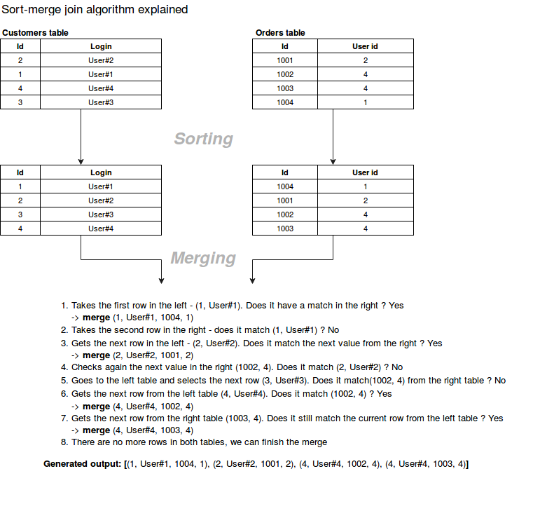
2. Phase 1: The Sort Phase

The first step is to ensure both tables are sorted on the join key. Since the tables are often too large to fit in memory, a disk-based sorting algorithm is required. As you may recall from the external sorting lesson (or will see in the implementation project LINK), this is precisely the job of the External Merge Sort algorithm.

An important optimization is to check if a table is already sorted on the join key. This can happen if:

• The table has a clustered B+ Tree index on the join attribute.
• The data is the output of a previous query plan operator that already produced a sorted result (this is known as an "interesting order").

If the data is already sorted, the sort phase for that table can be skipped entirely, providing a significant performance boost.

3. Phase 2: The Merge Phase

Once both relations are sorted, the merge phase begins. The logic is elegant and efficient. We use two pointers (or cursors), one for each relation, initialized to the first tuple. We then advance the pointers based on a comparison of the join keys.

Let's use pr to denote the pointer to the current tuple in relation R and ps for relation S.

1. If pr.key == ps.key: We have a match! We output a joined tuple. We then need to advance the pointers to check for more matches (we'll address the complication of duplicates shortly).
2. If pr.key < ps.key: Since the relations are sorted, we know pr cannot possibly match ps or any subsequent tuple in S. So, we advance pr.
3. If pr.key > ps.key: Symmetrically, we know ps cannot match pr, so we advance ps.

This process continues until one of the pointers reaches the end of its relation.

The following video from the CMU Database Group provides an excellent step-by-step walkthrough of this merge process.

Handling Duplicates: A Critical Detail

The simple pointer advancement logic gets tricky when duplicate join keys are present. For example, if we have multiple tuples in R with key 100 and multiple tuples in S with key 100, we must produce the full cross-product of these matching groups. A naive implementation might miss some of these pairs.

The CMU video you just watched hints at a "backtracking" mechanism. A more robust way to think about this, especially from an implementation perspective, is to use a co-grouping strategy.

The idea is:

1. When you find a match (pr.key == ps.key), you've identified a matching "group".
2. Scan forward in both R and S to find all adjacent tuples with that same key.
3. You now have two sets of tuples (one from R, one from S) that all share the same join key.
4. Compute the cross-product of these two small sets in memory.
5. Once done, reposition your main cursors (pr and ps) to the first tuple after these groups and continue the main merge loop.

This approach correctly handles many-to-many relationships without complex backtracking logic.

4. I/O Cost Analysis

The total I/O cost of a sort-merge join is the sum of the costs of its two phases. Let's assume we have B buffer pages available.

1. Sort Cost:
This is the cost of running external merge sort on both relations. Using the formula from our lectures, where a relation has P pages:
${\text{Cost}}_{\text{sort}}(P)=2P\times \left(1+\lceil {\log }_{B-1}\lceil \frac{P}{B}\rceil \rceil \right)$
So, the total sort cost is:
${\text{Cost}}_{\text{sort}}={\text{Cost}}_{\text{sort}}(M)+{\text{Cost}}_{\text{sort}}(N)$
For large tables, this sorting cost is the dominant part of the algorithm.

2. Merge Cost:

• Average Case: In the common scenario where duplicate keys are few and far between, the merge phase requires just a single scan of each sorted relation. The cost is simply $M+N$ I/Os.
• Worst Case: If all tuples in both relations have the same join key value, the algorithm degenerates. For each tuple in the outer relation's group, we'd have to scan the entire inner relation's group. This leads to a worst-case merge cost of $M\times N$ I/Os. This is highly unlikely in practice but is important to know.

Total Cost (Average Case):
$\text{Total Cost}\approx \underset{\text{Sort Phase}}{\underbrace{\left({\text{Cost}}_{\text{sort}}(M)+{\text{Cost}}_{\text{sort}}(N)\right)}}+\underset{\text{Merge Phase}}{\underbrace{(M+N)}}$

Let's see how this stacks up against the other algorithms.

Conclusion

We've now added a powerful tool to our query execution toolbox. Sort-Merge Join is an excellent general-purpose algorithm for joining large tables, especially when a suitable index for an Index Nested Loop Join is not available.

Key Takeaways:

• Two-Phase Algorithm: Sort-Merge join consists of a Sort Phase (using external merge sort) and a Merge Phase (using a synchronized scan with two pointers).
• I/O Cost: The cost is dominated by the initial sort, with an average-case total of roughly ${\text{Cost}}_{\text{sort}}(M)+{\text{Cost}}_{\text{sort}}(N)+M+N$.
• Duplicate Handling: Correctly joining tuples with duplicate keys is non-trivial and requires a robust strategy like co-grouping to ensure correctness.
• "Interesting Orders": A major advantage of this algorithm is that its output is sorted on the join key, which may eliminate the need for a separate ORDER BY operation later in the query plan.

Preview of the Next Lesson

While Sort-Merge join is a huge improvement over nested loop joins for large tables, the CMU video hinted that there's often an even faster method: Hash Join. In our next lesson, we will explore the Grace Hash Join algorithm, which uses hashing to partition relations into memory-sized buckets, replacing the expensive sorting phase with a potentially cheaper hashing phase.