Two-Pass Grace Hash Join Implementation

1. The Core Idea: In-Memory Hash Join

Let's start with the simplest case: one of the tables, which we'll call the "build" (or outer) table, is small enough to fit entirely in memory. The algorithm works in two phases:

1. Build Phase: Scan the entire build relation (let's say R) and use its tuples to build an in-memory hash table. The keys of this hash table are the join key attributes.
2. Probe Phase: Scan the "probe" (or inner) relation (S), one tuple at a time. For each tuple from S, hash its join key and probe the in-memory hash table to find matching tuples from R. If a match is found, output the joined tuple.

This approach is extremely fast because it only requires one full scan of each table, and hash table lookups are, on average, an O(1) operation.

This simple hash join is fantastic, but it relies on a critical assumption: the build table's hash table fits in memory. What happens when both tables are enormous, and neither can be held in memory? This is the problem that the Grace Hash Join solves.

2. Grace Hash Join: Hashing for Out-of-Core Joins

The Grace Hash Join (also called Partitioned Hash Join) is a two-pass algorithm that uses a clever "divide and conquer" strategy. Instead of trying to join the entire tables at once, it first partitions them into smaller, corresponding buckets that can fit in memory.

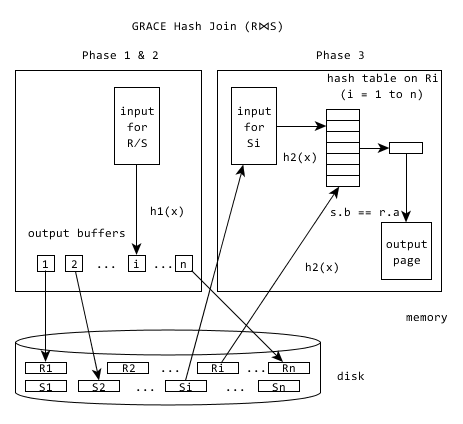
Let's break down the two passes.

Pass 1: The Partitioning Phase

The goal of this pass is to split both relations, R and S, into smaller files (partitions or buckets) on disk.

1. Allocate B-1 buffer pages as output buffers for B-1 partitions, and one buffer page as an input buffer.
2. Read relation R page by page. For each tuple in the input buffer, apply a hash function h1 to its join key.
3. The result of h1(key) determines which of the B-1 partitions the tuple belongs to. Move the tuple to the corresponding output buffer.
4. When an output buffer becomes full, write it to a partition file on disk.
5. Repeat this entire process for relation S using the exact same hash function h1.

The key insight here is that any two tuples r ∈ R and s ∈ S that could possibly join (i.e., r.key == s.key) are guaranteed to be hashed to the same partition number. We've effectively divided one massive join problem into B-1 smaller, independent join problems.

Pass 2: The Probing Phase

Now that the data is partitioned, the second pass joins each pair of corresponding partitions.

1. For each partition i (from 0 to B-2):
   • Read the entire partition R_i into memory and build an in-memory hash table using a different hash function, h2. (Using a different function helps avoid issues if h1 had bad collision properties).
   • Read the corresponding partition S_i page by page.
   • For each tuple in S_i, use h2 to probe the in-memory hash table for matches from R_i.
   • Output any matching pairs.

Since each partition R_i was created to be small enough to fit in memory, this second phase is just a series of in-memory hash joins.

This process can be tricky to visualize. The following animation makes it much clearer.

For a more detailed explanation and some historical context on the name "Grace" Hash Join, let's return to the CMU lecture.

3. Cost Analysis and Real-World Implementation

Understanding the I/O cost of Grace Hash Join is straightforward and reveals why it's so powerful.

• Partitioning Phase: We read every page of R and S once, and we write every page of R and S once to disk partitions.
  • Cost: 2 * (M + N) I/Os.
• Probing Phase: We read every page of the R and S partitions back into memory once to perform the joins.
  • Cost: M + N I/Os.
• Total Cost: 3 * (M + N) I/Os.

This linear cost is typically much lower than the super-linear cost of external sorting required by Sort-Merge Join.

A Look Inside a Real System: ClickHouse

Your preference for technical blogs from developers gives us a great opportunity. Let's see how the Grace Hash Join is implemented and used in ClickHouse, a popular high-performance analytical database. This gives an engineering perspective on the trade-offs involved.

Conclusion

You've now learned the mechanics of one of the most important algorithms in database query processing. The Grace Hash Join is the workhorse for joining massive tables when no indexes are available.

Key Takeaways:

• Two-Pass Design: Grace Hash Join consists of a Partitioning Phase to divide large tables into smaller, corresponding disk-based buckets, and a Probing Phase that performs in-memory hash joins on each bucket pair.
• I/O Cost: The total cost is 3 * (M + N), which is linear with respect to the size of the tables and often superior to the cost of Sort-Merge Join.
• Core Principle: It turns a large, out-of-core problem into a series of smaller, in-memory problems using hashing as the partitioning key.
• Skew Handling: Robust implementations must be prepared to handle data skew (where one partition is still too large) by using recursive partitioning.

Preview of the Next Lesson

We have now examined several join algorithms: Block Nested Loop, Index Nested Loop, Sort-Merge, and Hash Join. Each has its strengths and weaknesses. The next logical question is: how does a database system choose which one to use for a given query? In our next lesson, we will compare the performance trade-offs between these strategies and lay the groundwork for understanding query optimization.