Big O Complexity of Algorithms

What is Time Complexity?

First, let's establish what time complexity is not. It's not about measuring how many seconds your code takes to run on your laptop. That time can change dramatically based on your computer's speed, the programming language, and other factors.

Instead, time complexity describes the relationship between the size of the input to a problem (which we'll call n) and the number of operations the algorithm performs. It measures how the runtime scales as the input n gets larger.

To get a clear intuition for this, let's watch a short segment from the "Strivers A2Z DSA Course".

As the video explains, we need a standardized way to describe this rate of growth. This is where Big O notation comes in.

The Language of Efficiency: Big O Notation

Big O notation is the mathematical language used in computer science to describe the performance or complexity of an algorithm. When we analyze an algorithm, we're usually interested in its worst-case performance, as this gives us an upper bound on how long it might take.

To make the analysis simpler and more general, Big O notation follows three key principles:

1. Always analyze the worst-case scenario: We want a guarantee that our algorithm will be fast enough, even for the trickiest test cases.
2. Ignore constants: An algorithm that takes 3n operations and one that takes n operations are both considered to have a linear, or O(n), complexity. The constant factor (3) becomes insignificant as n grows very large.
3. Ignore lower-order terms: If an algorithm takes $n^2+n$ operations, we only care about the fastest-growing term, $n^2$. For large n, the $n^2$ part dominates so completely that the n part is negligible. So, we simplify this to $O(n^2)$.

The same video explains these rules with clear examples.

To solidify this, let's look at a textual explanation with some more examples. The following reading from a Codeforces blog post gives a concise definition of Big O.

Analyzing Code Complexity

Now for the practical part: how do you look at a piece of C++ code and figure out its Big O complexity? The most common way is to analyze the loops.

• A single for loop that runs n times performs n iterations. If the work inside the loop takes constant time, the total complexity is $O(n)$.

  for (int i = 0; i < n; i++) {
      // O(1) constant time work
  }
  

• Two separate, sequential loops have their complexities added. A loop that runs N times followed by a loop that runs M times results in $O(N+M)$ complexity.

  for (int i = 0; i < N; i++) { /* O(1) work */ }
  for (int j = 0; j < M; j++) { /* O(1) work */ }
  

• Nested loops have their complexities multiplied. A loop that runs n times with another loop inside it that also runs n times results in $O(n\times n)=O(n^2)$.

  for (int i = 0; i < n; i++) {
      for (int j = 0; j < n; j++) {
          // O(1) constant time work
      }
  }
  

Let's dive into some more detailed examples from the Codeforces blog.

A Hierarchy of Common Complexities

Not all complexities are created equal. An $O(n^2)$ algorithm will be much slower than an $O(n)$ one for large inputs. It's crucial to have a mental picture of how these complexities compare.

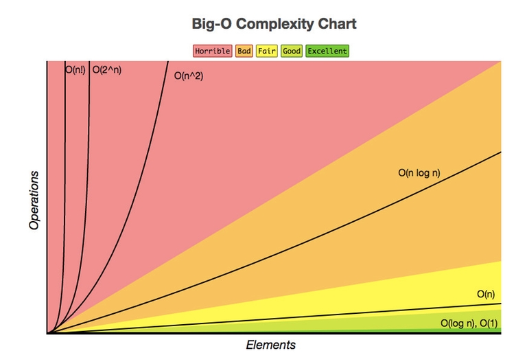
Here's a list of common complexities, from fastest (excellent) to slowest (horrible):

• $O(1)$ - Constant: The runtime doesn't depend on the input size. (e.g., accessing an array element at a known index).
• $O(\log n)$ - Logarithmic: The runtime grows very slowly. If n doubles, the runtime increases by a small constant amount. (e.g., Binary Search).
• $O(n)$ - Linear: The runtime grows proportionally to the input size. (e.g., finding the maximum element in an unsorted array).
• $O(n\log n)$ - Log-linear: A very common and efficient complexity for sorting algorithms. (std::sort in C++ is typically $O(n\log n)$).
• $O(n^2)$ - Quadratic: Runtime grows with the square of the input size. Often involves nested loops over the input. (e.g., Bubble Sort, simple nested for loops).
• $O(2^n)$ - Exponential: Becomes extremely slow even for small n. Often seen in problems that involve generating all subsets of a set.
• $O(n!)$ - Factorial: The slowest of all. Usually associated with generating all permutations of a set.

You already know about binary search and sorting. Let's see how their complexities are formally derived.

What About Space Complexity?

Besides time, we also care about the memory an algorithm uses. Space complexity measures the amount of memory an algorithm needs, as a function of the input size n. We usually focus on auxiliary space complexity, which is the extra space used by the algorithm beyond the space required to store the input itself.

• An algorithm that only uses a few variables, regardless of the input size, has $O(1)$ space complexity.
• An algorithm that creates a new array or vector of the same size as the input has $O(n)$ space complexity.
• A recursive function that calls itself n times before returning might use $O(n)$ space on the call stack.

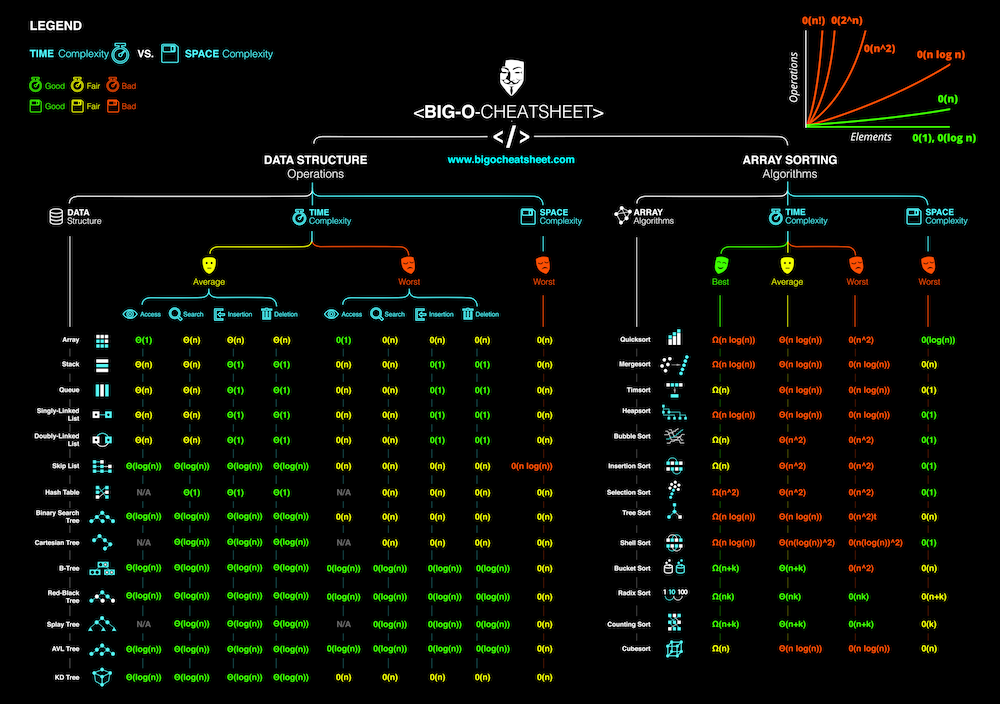
This "Big-O Cheat Sheet" is an invaluable resource that summarizes the time and space complexity for many common data structures and algorithms. It's a great reference to bookmark.

The Most Important Trick for Competitive Programmers

Here is the key takeaway that will immediately elevate your problem-solving strategy. On most competitive programming platforms like Codeforces, a modern server can execute approximately 10⁸ (100 million) operations in one second.

This single fact allows you to work backward from the problem constraints to figure out what time complexity is required.

Let's watch a short video that explains this powerful "reverse trick".

Here's a quick summary of those N-rules for a 1-second time limit:

• If $N\le 20$: An $O(2^N)$ or $O(N!)$ solution might pass.
• If $N\le 300$: An $O(N^3)$ solution is likely fine. ($300^3\approx 2.7\times 10^7$)
• If $N\le 5000$: An $O(N^2)$ solution should pass. ($5000^2=2.5\times 10^7$)
• If $N\le 10^5-10^6$: You need an $O(N\log N)$ or $O(N)$ solution. $O(N^2)$ is definitely too slow.
• If $N>10^7$: You likely need an $O(\log N)$ or $O(1)$ solution. Even $O(N)$ will be too slow.

This is arguably the most important skill in competitive programming strategy. Before you even think about an algorithm, look at the constraints for N. They are a massive hint from the problem setter about the expected solution complexity.

Conclusion

In this lesson, you've taken the first and most fundamental step toward thinking like an expert competitive programmer.

Here are the key takeaways:

• Time complexity describes how an algorithm's runtime scales with input size, not its absolute speed in seconds.
• Big O notation is the standard for expressing this, focusing on the worst-case and ignoring constants and lower-order terms.
• You can analyze code, particularly loops, to determine its Big O complexity ($O(n)$, $O(n^2)$, etc.).
• Space complexity measures the auxiliary memory used by an algorithm.
• The crucial insight for competitive programming is that you can use the problem's input constraints and the "10⁸ operations per second" rule to deduce the required time complexity before you start coding.

In the next lesson, we will put this last point into practice. We'll look at several Codeforces problems and focus solely on their constraints to predict the required time complexity, a skill that will guide your choice of algorithm and save you countless hours of debugging TLE solutions.