Estimating Time Complexity: N-Rules for Codeforces

In our previous lesson, we introduced the foundational concepts of time complexity and Big O notation. Most importantly, we unveiled the single most powerful strategic tool in a competitive programmer's arsenal: the "10⁸ operations per second" rule. This rule allows you to work backward from a problem's constraints to determine the required efficiency of your solution.

Today, we will master this skill. You will learn to glance at the input size, N, and immediately understand the "shape" of the algorithm the problem setter expects. This isn't just a trick; it's the first and most critical step in designing a solution that will pass the time limit, a habit that separates advancing programmers from those stuck on "Time Limit Exceeded" errors.

The Programmer's Compass: A Guide to Complexity Constraints

Think of the problem constraints as a direct hint from the problem setter. When they say $N \leq 1 0^{5}$ , they are telling you that any solution slower than $O (N lo g N)$ is almost certain to fail. Let's start by solidifying the relationship between the input size and the required complexity.

First, let's revisit the visual representation of how different complexity classes grow.

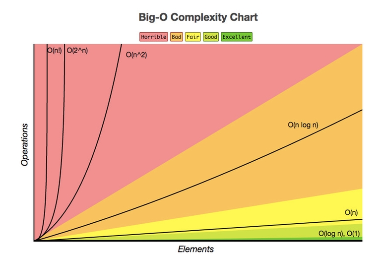
This chart vividly shows why choosing the right complexity matters. As the number of elements (`N`) on the x-axis increases, the number of operations for "Horrible" complexities like $O(N^2)$ and $O(2^N)$ skyrockets, while "Excellent" and "Good" complexities like $O(\log N)$ and $O(N)$ grow much more slowly.

Based on the ~10⁸ operations-per-second rule, we can create a "cheat sheet" that maps input sizes to viable time complexities. The following reading from a training slide deck provides a concise and effective version of these rules.

Introduction to Competitive Programming, Big-O

These slides from the Hong Kong Olympiad in Informatics (HKOI) training material provide a clear, practical table mapping input sizes to required complexities for a 1-second time limit.

Please review slides 46, 47, and 48. Focus on the table presented on slide 47. These are the "N-rules" that you should aim to internalize.

Let's summarize and slightly expand upon that table. For a typical 1-second time limit on Codeforces:

Input Constraint (N)	Required Complexity	Common Algorithms / Patterns
$N \leq 10 - 12$	$O (N!)$	Permutations of a small set
$N \leq 20 - 22$	$O (2^{N})$	Generating all subsets (bitmask DP)
$N \leq 100$	$O (N^{4})$	Four nested loops
$N \leq 400$	$O (N^{3})$	Three nested loops (e.g., Floyd-Warshall)
$N \leq 5000$	$O (N^{2})$	Two nested loops, basic DP
$N \leq 1 0^{5} - 1 0^{6}$	$O (N lo g N)$	Sorting, binary search on the answer, segment trees
$N \leq 1 0^{7}$	$O (N)$	Linear scan, prefix sums, two pointers
$N \geq 1 0^{9}$	$O (lo g N)$ or $O (1)$	Binary search, math formulas

This table will become your most trusted guide. Before writing any code, your first thought should be: "Where does my N fit in this table?"

Case Study: A Tale of Two Sorts

Let's make this concrete. Imagine a problem asks you to sort an array where $N \leq 1 0^{6}$ . You know two sorting algorithms: Bubble Sort, which is $O (N^{2})$ , and std::sort (based on Introsort), which is $O (N lo g N)$ .

Let's do the math:

Bubble Sort ( $O (N^{2})$ ):
- For $N = 1 0^{6}$ , the number of operations is roughly $(1 0^{6})^{2} = 1 0^{12}$ .
- Since a judge can do about $1 0^{8}$ operations per second, this would take $\frac{1 0 ^{12}}{1 0 ^{8}} = 1 0^{4}$ seconds, which is almost 3 hours. This is a guaranteed Time Limit Exceeded (TLE).
std::sort ( $O (N lo g N)$ ):
- For $N = 1 0^{6}$ , the number of operations is roughly $1 0^{6} \times lo g_{2} (1 0^{6})$ .
- $lo g_{2} (1 0^{6})$ is approximately 20 (since $2^{20} \approx 1 0^{6}$ ).
- Total operations: $1 0^{6} \times 20 = 2 \times 1 0^{7}$ .
- This is well under our $1 0^{8}$ budget and will pass comfortably within the 1-second time limit.

The following video walks through this exact scenario, providing a clear, practical demonstration of why choosing the right algorithm based on constraints is non-negotiable.

Time Limit Exceeded- How To Avoid TLE ? | Trick To Pass All Test Cases In Competitive Programming

This video segment provides a clear, step-by-step calculation showing why Bubble Sort would fail and Merge Sort (another O(N log N) algorithm) would pass for an input size of 10^6.

Watch the section explaining the choice between two algorithms. Pay attention to how the Big O complexity is translated into a concrete number of operations to estimate the runtime. Watch from the exercise.

Reading the Fine Print: Multiple Inputs and Test Cases

Codeforces problems often add a couple of twists to this analysis.

Multiple Input Variables

Sometimes, the complexity isn't just a function of N. You might have N and M, or R and C (rows and columns). The logic remains the same. If the constraints are $N, M \leq 1000$ , an $O (N \cdot M)$ solution (like iterating through a grid) would involve about $1000 \times 1000 = 1 0^{6}$ operations, which is perfectly fine. However, if $N, M \leq 1 0^{5}$ , an $O (N \cdot M)$ approach is impossible, and you'd need something closer to $O (N + M)$ .

"Sum of N over all test cases"

This is a very common and important constraint pattern on Codeforces. A problem might have constraints like:

Number of test cases, $t \leq 1 0^{4}$
Input size per test case, $N \leq 1 0^{5}$
Time Limit: 1 second

A beginner might multiply the worst cases: $t \times N = 1 0^{4} \times 1 0^{5} = 1 0^{9}$ , and conclude that even an $O (N)$ solution per test case is too slow. However, these problems almost always include an additional, crucial line:

"The sum of N over all test cases does not exceed $2 \cdot 1 0^{5}$ ."

This statement overrides the individual limits. It tells you that even though a single test case could have $N = 1 0^{5}$ , you won't get many such large cases. The total work across all test cases for an $O (N)$ solution is bounded by the sum, not the product. If the total $N$ is $2 \cdot 1 0^{5}$ , an $O (N)$ solution will perform about $2 \cdot 1 0^{5}$ operations in total, which is very fast.

The following reading from the Codeforces blog we looked at last time explains this point perfectly.

A Time Complexity Guide

This section of the guide explains the crucial difference between worst-case complexity per test case and the total complexity when the "sum of N" is constrained.

Read the last paragraph of the section "Time Complexity during problem solving". Focus on the example provided, from this explanation of handling multiple test cases.

Test Your Intuition

Let's do a quick drill. For each set of constraints below (assuming a 1s time limit), what is the most likely required time complexity?

Constraints: $1 \leq N \leq 22$

Answer
**$O(2^N)$ or $O(2^N \cdot N)$**. This range is the classic signal for a solution that involves iterating through all subsets of `N` elements, often using bitmasking. An $O(N!)$ solution would be too slow as $22!$ is enormous.

2. **Constraints:** $1 \le N \le 10^5$, array values are up to $10^9$.

Answer

**$O(N \log N)$ or $O(N)$**. This is the most common range in Div2 problems. $O(N^2)$ is too slow. You should immediately think of sorting, binary search, two pointers, or other linear-time data structures.

3. **Constraints:** $1 \le N \le 300$

Answer

**$O(N^3)$**. With $N=300$, $N^3$ is $2.7 \cdot 10^7$, which fits snugly within the time limit. This is a strong hint for algorithms like Floyd-Warshall or DP with three state variables. An $O(N^2)$ solution would also pass easily.

4. **Constraints:** $1 \le N \le 10^{12}$

Answer

**$O(\log N)$ or $O(1)$**. An input this large means you cannot iterate over it. The solution must involve a mathematical formula ($O(1)$), binary search on the answer space ($O(\log N)$), or perhaps matrix exponentiation ($O(k^3 \log N)$ where `k` is small).

5. **Constraints:** $t$ testcases, $1 \le N, M \le 1000$, sum of $N \cdot M$ over all testcases $\le 2 \cdot 10^5$.

Answer

**$O(N \cdot M)$** per test case. Even though a single test case could be $1000 \times 1000 = 10^6$, the "sum of" constraint tells us the total work for a grid traversal across all test cases is manageable.

Conclusion

In this lesson, we've transformed a theoretical concept into a powerful, practical problem-solving weapon. By internalizing the "N-rules," you've learned how to decode a problem's constraints to instantly narrow down the field of possible algorithms.

Here are the key takeaways:

Constraints are your guide: Before thinking about code, always check the input size to determine the required time complexity.
Internalize the N-rules: Keep the mapping of N to complexity (e.g., $N \leq 1 0^{5} ⟹ O (N lo g N)$ ) at the front of your mind.
Beware the fine print: Pay close attention to multiple variables and especially the "sum of N over all test cases" clause, as it radically changes the analysis.

This strategic analysis is the very first thing an expert programmer does. Now that you know how to determine what kind of solution is needed (e.g., an $O (N lo g N)$ one), the next question is: how do you come up with one and trust that it's correct?

In our next lesson, we will explore the vital role of a naive (brute-force) solution. It may sound counterintuitive, but a slow, simple solution is one of your best tools for developing and verifying a fast, optimized one.

Recommended resources

The Programmer's Compass: A Guide to Complexity Constraints

Case Study: A Tale of Two Sorts

Reading the Fine Print: Multiple Inputs and Test Cases

Multiple Input Variables

"Sum of N over all test cases"

Test Your Intuition

Conclusion