Calculating Historical Volatility

1. The Three Steps to Historical Volatility

Historical volatility (HV) is a backward-looking measure that quantifies how much an asset's price has fluctuated over a specific period. It is, fundamentally, the standard deviation of the asset's returns. The calculation process involves three main steps:

1. Calculate daily returns: Determine the day-over-day percentage change in price.
2. Calculate the standard deviation: Measure the dispersion of these returns.
3. Annualize the result: Scale the daily volatility to an annual figure to make it comparable with other financial metrics, like the implied volatility (IV) of options.

Let's break these down.

Step 1: Calculating Logarithmic Returns

While you can use simple percentage change, it is standard practice in quantitative finance to use logarithmic (or "log") returns. They have several desirable mathematical properties, such as being time-additive. The formula is:

${\text{Log Return}}_t=\ln \left(\frac{{\text{Price}}_t}{{\text{Price}}_{t-1}}\right)$

In Python with Pandas, this is straightforward. We can get a demonstration from the following video.

As you saw, the code is simply:
log_returns = np.log(df['Close'] / df['Close'].shift(1))

Step 2: Calculating the Standard Deviation

With a series of daily log returns, the next step is to calculate their standard deviation using the .std() method in Pandas.

However, there's a subtle but important detail here concerning the "delta degrees of freedom" (ddof).

• Pandas' .std() function defaults to ddof=1, calculating the sample standard deviation.
• NumPy's .std() function defaults to ddof=0, calculating the population standard deviation.

Since our historical data is just a sample of all possible price movements, the sample standard deviation (ddof=1) is the appropriate choice. This is a key detail for building a "foolproof" system, as using the wrong standard deviation can lead to small but meaningful differences in your calculations.

Step 3: Annualizing the Volatility

The standard deviation we've calculated is a daily volatility. To make it comparable to option-implied volatility, we must annualize it. This is done by multiplying the daily volatility by the square root of the number of trading days in a year, which is typically assumed to be 252.

Let's see this final step implemented in code.

2. Calculating Rolling Historical Volatility

A single HV number for an entire multi-year dataset isn't very useful for generating timely trade signals. We need to know what the volatility has been recently. To do this, we calculate historical volatility over a rolling window (e.g., the last 20, 30, or 60 trading days).

Pandas makes this incredibly easy with the .rolling() method. We can chain it with .std() to get a rolling standard deviation, which we then annualize.

For a complete function that pulls these concepts together, let's refer to an article from PyQuant News.

Here is a Python function adapted from that example, which you can add to a new file in your project, framework/analytics.py:

# In framework/analytics.py

import numpy as np
import pandas as pd
import math

def calculate_historical_volatility(
    price_data: pd.Series, 
    window: int = 21, 
    trading_periods: int = 252
) -> pd.Series:
    """
    Calculates the annualized historical volatility over a rolling window.
    
    Args:
        price_data (pd.Series): A pandas Series of closing prices, indexed by date.
        window (int): The rolling window period in days. Default is 21 (approx 1 month).
        trading_periods (int): The number of trading periods in a year. Default is 252.
        
    Returns:
        pd.Series: A pandas Series of annualized historical volatility.
    """
    if not isinstance(price_data, pd.Series):
        raise TypeError("price_data must be a pandas Series.")
        
    # Calculate logarithmic returns
    log_returns = np.log(price_data / price_data.shift(1))
    
    # Calculate rolling standard deviation of log returns
    rolling_std = log_returns.rolling(window=window, center=False).std()
    
    # Annualize the standard deviation
    annualized_volatility = rolling_std * math.sqrt(trading_periods)
    
    return annualized_volatility.dropna()

Note: A common window is 21 days, representing the approximate number of trading days in a month.

3. A More Robust Approach: SMA vs. EWMA Volatility

The .rolling() function calculates a Simple Moving Average (SMA) of the volatility. Every data point in the window is weighted equally. This has a significant drawback known as the "ghosting" or "leverage effect." A single large price shock will keep the calculated volatility high for the entire duration of the window, and then cause a sudden, artificial drop when it finally falls out of the window.

A more robust and responsive method is the Exponentially Weighted Moving Average (EWMA). EWMA assigns more weight to recent data, causing the volatility estimate to react faster to new information and decay more smoothly from old shocks.

Fortunately, Pandas also has a built-in method for this: .ewm(). We can modify our function to optionally use this more advanced method. The span parameter in .ewm() is roughly comparable to the window in .rolling().

Here is an enhanced version of our function. For your "foolproof" system, using the ewma method is generally preferable.

# In framework/analytics.py (updated function)

def calculate_historical_volatility(
    price_data: pd.Series, 
    window: int = 21, 
    trading_periods: int = 252,
    method: str = 'ewma' # 'sma' or 'ewma'
) -> pd.Series:
    """
    Calculates the annualized historical volatility over a rolling window.
    
    Args:
        price_data (pd.Series): A pandas Series of closing prices, indexed by date.
        window (int): The rolling window period (for sma) or span (for ewma).
        trading_periods (int): The number of trading periods in a year.
        method (str): 'sma' for simple moving average or 'ewma' for exponentially
                      weighted moving average.
                      
    Returns:
        pd.Series: A pandas Series of annualized historical volatility.
    """
    if not isinstance(price_data, pd.Series):
        raise TypeError("price_data must be a pandas Series.")
        
    log_returns = np.log(price_data / price_data.shift(1))
    
    if method == 'sma':
        rolling_std = log_returns.rolling(window=window, center=False).std()
    elif method == 'ewma':
        # Using ewm().std() is more responsive to recent volatility changes.
        rolling_std = log_returns.ewm(span=window, min_periods=window, center=False).std()
    else:
        raise ValueError("Method must be 'sma' or 'ewma'.")
        
    annualized_volatility = rolling_std * math.sqrt(trading_periods)
    
    return annualized_volatility.dropna()

4. Beyond Close-to-Close: A Glimpse at Other Methods

The method we've implemented, based on the standard deviation of close-to-close log returns, is the most common form of HV. However, it's not the only one. It can miss significant price swings that occur during the trading day but are not reflected in the closing price.

More advanced estimators exist to capture this intraday volatility:

• Parkinson: Uses the day's high and low prices.
• Garman-Klass: Extends Parkinson by also incorporating the open and close prices.

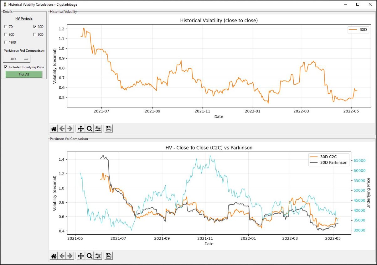
While exploring these is beyond our immediate scope, it's valuable to know they exist. For building our first signal generator, the EWMA of close-to-close returns is a robust and excellent starting point.

Conclusion

You have now built a practical and robust function to calculate historical volatility, a fundamental metric in quantitative trading. This function is a tangible asset for your trading framework.

Key Takeaways:

• Historical Volatility is the annualized standard deviation of returns, typically log returns.
• The calculation involves three steps: compute returns, find the rolling standard deviation, and annualize by multiplying by sqrt(252).
• Using an Exponentially Weighted Moving Average (.ewm()) is often superior to a Simple Moving Average (.rolling()) as it is more responsive to recent data and avoids the "ghosting effect."
• Subtle details, like using the sample standard deviation (ddof=1), are important for numerical accuracy.

Preview of the Next Lesson:
With our calculate_historical_volatility function ready, we have one of the two key inputs for our volatility-based signal. In the next lesson, we will put this to use by implementing a concrete signal generator that compares this historical volatility to implied volatility, producing the 'ENTRY' or 'NO_ENTRY' signals our framework needs.