Hello and welcome to the first lesson in our module on efficient attention mechanisms.
In the previous module, we assembled the complete, modern Transformer block, understanding how components like RMSNorm, SwiGLU, RoPE, and Pre-LN work together to create a stable and powerful architecture.
Today, we shift our focus from individual components to a major system-level challenge: the cost of inference. As you'll recall from our earlier lessons, autoregressive models like GPT generate text one token at a time. To avoid massive recomputation, they use a KV Cache. While this trick saves computation, it comes at a steep price in memory. This memory cost is the primary bottleneck for enabling long context windows and is the motivation behind many modern architectural innovations.
Our learning outcome for this lesson is to quantify the KV cache memory cost for standard multi-head attention as a function of layers, heads, and sequence length. By the end of this lesson, you will be able to calculate the GPU memory required for the KV cache of any standard Transformer model and understand why this has driven the development of more efficient attention mechanisms.
1. Recap: The Purpose of the KV Cache
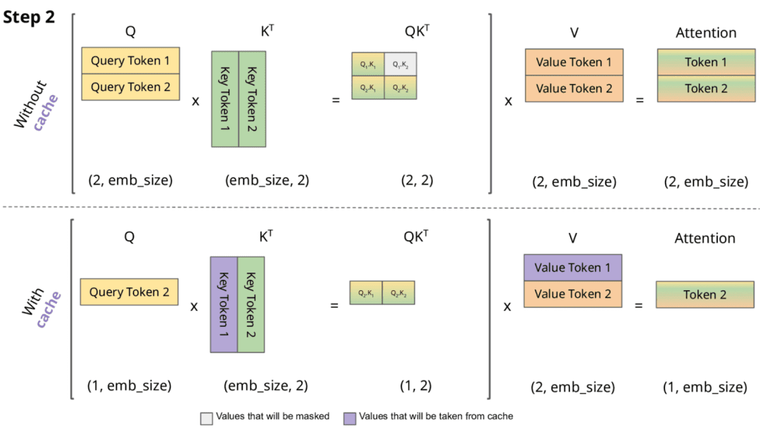
Let's begin with a quick review. During autoregressive generation, a model predicts the next token based on all the tokens it has seen so far. For example, to predict the token following "The next day is", the model computes attention scores between "is" and all preceding tokens ("The", "next", "day").
Without a cache, when the model then predicts the token after "The next day is bright", it would have to recompute the Key (K) and Value (V) vectors for "The", "next", "day", and "is" all over again. This is computationally wasteful.
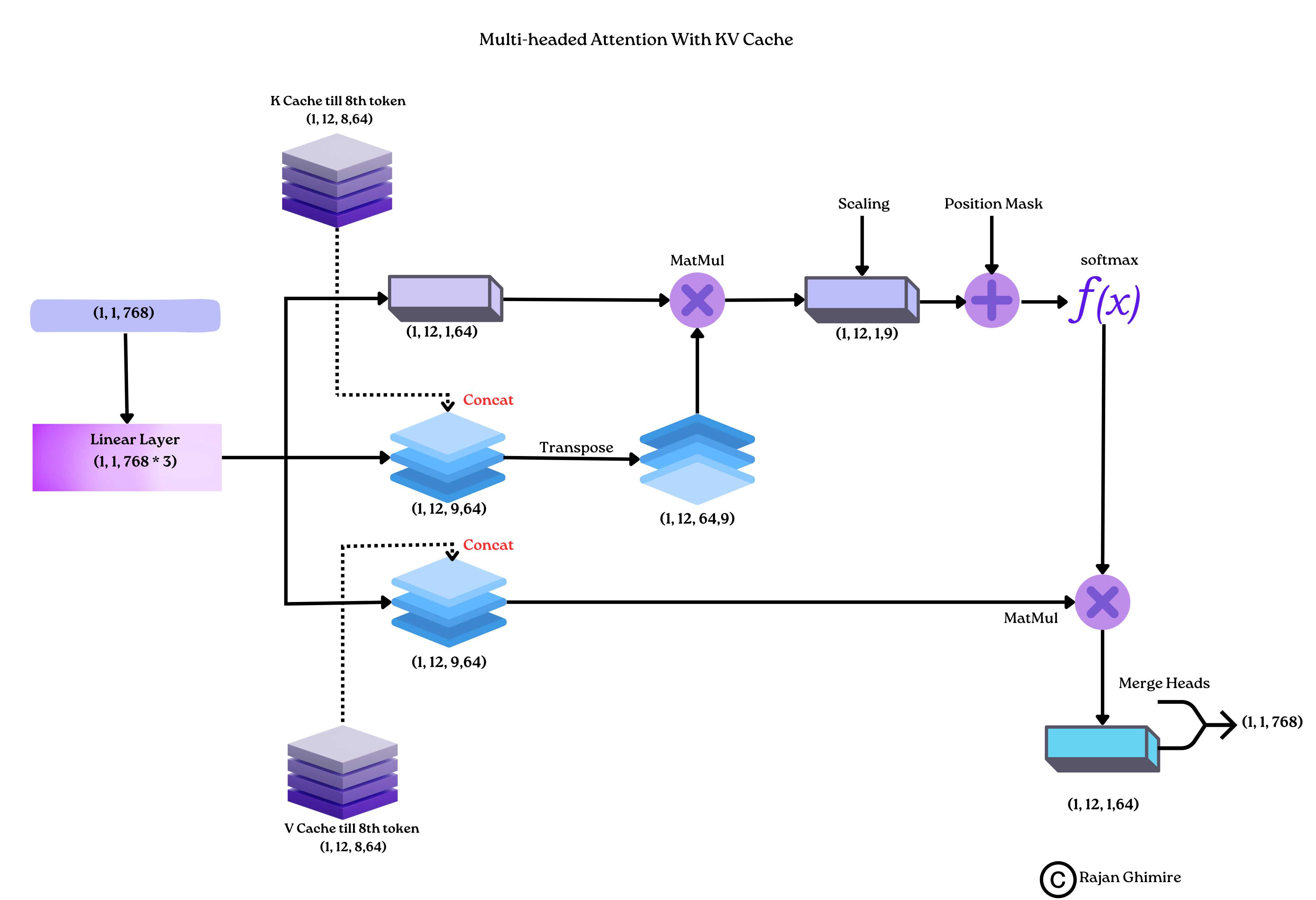
The KV cache solves this by storing the K and V vectors for all tokens in the sequence. At each new step, the model only needs to compute the K and V vectors for the newest token and append them to the cache.
To quickly refresh your memory on this process, the following video provides a concise explanation.
The KV Cache: Memory Usage in Transformers
The video 'The KV Cache: Memory Usage in Transformers' from the Efficient NLP channel gives a clear overview of why the cache is needed and how it works.
Please watch from 04:07 to 04:42. Focus on how the model only computes the key and value for the new token and appends it to the cached matrices.
This caching strategy transforms the computational complexity of attention from being quadratic with respect to sequence length to linear. However, this computational saving comes at the cost of storing an ever-growing cache in the GPU's memory.
2. Deriving the KV Cache Memory Formula
Our goal is to derive a formula to calculate the size of this cache. We can build it up from first principles.
Let's define the key dimensions of a Transformer model:
B: Batch size (number of sequences processed in parallel)S: Sequence length (number of tokens in the sequence)L: Number of attention layers in the modelN: Number of attention heads per layerH: Dimension of each attention head (d_head)
The total hidden dimension of the model, D (or d_model), is N * H.
-
Cache for one token, one head, one layer: For a single token, each attention head computes one Key vector and one Value vector. Each of these vectors has a dimension of
H. Therefore, we need to store2 * Hfloating-point numbers. -
Across all heads: Since there are
Nheads in the layer, the storage for one token in one layer becomes2 * N * H. As we knowD = N * H, this simplifies to2 * Dnumbers per token per layer. -
Across all layers: The model has
Llayers, and each has its own KV cache. So, the storage for a single token across all layers isL * (2 * D)numbers. -
For the entire sequence: The cache must store the K and V vectors for every token in the sequence of length
S. So, we multiply byS:S * L * 2 * Dnumbers. -
For the entire batch: If we are processing a batch of
Bsequences simultaneously, the total storage isB * S * L * 2 * Dnumbers. -
Converting to Bytes: Finally, we must account for the precision of these numbers. During inference, models typically use 16-bit floating-point formats like FP16 or BF16, where each number requires 2 bytes of storage.
This gives us our final formula for the total memory size of the KV cache in bytes:
where the first 2 accounts for storing both K and V matrices.
The following article from NVIDIA's developer blog presents this exact formula.
Mastering LLM Techniques: Inference Optimization
This article, 'Mastering LLM Techniques: Inference Optimization', provides a clear breakdown of LLM memory requirements and confirms our derived formula.
Please read the sections titled 'LLM memory requirement' and the subsequent section presenting the formula for the 'Total size of KV cache in bytes'. Notice how it matches our step-by-step derivation.
This formula reveals a critical relationship: the KV cache memory requirement grows linearly with both the batch size (B) and the sequence length (S). This is why handling long contexts is so memory-intensive.
3. A Worked Example: Calculating the Cost
Now let's apply this formula to a real-world model to see just how large this cache can become.
The video we watched earlier provides an excellent worked example for a 30-billion parameter model.
The KV Cache: Memory Usage in Transformers
Let's return to the 'The KV Cache: Memory Usage in Transformers' video to see the formula in action.
Watch from 05:55 to 07:39. Pay close attention to how each variable in the formula (precision, layers, dimension, sequence length, batch size) is substituted with concrete numbers to arrive at the final memory cost.
As the video demonstrates, for a 30B model with a batch size of 128 and a sequence length of 1024, the KV cache requires 180 GB of memory. This is three times the memory needed for the model weights themselves (60 GB)!
Let's do another example, this time with the DeepSeek-V3 base model, which is a focus of this course. We can use the parameters discussed in another one of our reference videos.
B(batch_size) = 1S(sequence_length) = 100,000 (a very long context)L(num_layers) = 61D(hidden_size) =N * H= 128 heads * 128 dim/head = 16,384precision_in_bytes= 2 (for FP16)
Plugging these into our formula:
That's approximately 400 GB for a single sequence! This massive memory footprint makes it clear why optimizing the KV cache is not just a minor improvement but a fundamental necessity for deploying large models with long context capabilities.
4. Practical Implications: GPU Capacity Limits
This calculation has a direct impact on real-world system design. The memory of a GPU is finite. For example, a high-end NVIDIA A100 GPU comes with 40 GB or 80 GB of VRAM.
The following article walks through this exact thought process: given a model's weight size and KV cache requirements, how many tokens can you actually fit on a given set of GPUs?
Transformer Inference Arithmetic
The article 'Transformer Inference Arithmetic' connects our memory calculation to the practical problem of hardware capacity.
Please read the section titled 'capacity'. It calculates the memory for model weights, subtracts that from the total available GPU memory, and then uses the remaining memory to determine the maximum size of the KV cache.
The article shows that for a 52B parameter model, which requires 104 GB for its weights, you would need at least three 40GB A100 GPUs. This leaves only 16 GB of VRAM for the KV cache, which severely limits the batch size and sequence length you can serve. This is the memory bottleneck in action.
Conclusion
In this lesson, we moved from a conceptual understanding of the KV cache to a quantitative one.
Key Takeaways:
- The KV cache avoids redundant computation during autoregressive inference, but it consumes a significant amount of GPU memory.
- The memory cost can be quantified with the formula:
Total Cache Size (Bytes) =batch_size×sequence_length× 2 ×num_layers×hidden_size×precision_in_bytes - This memory cost grows linearly with sequence length, making it the primary obstacle to achieving very long context windows.
- For large models, the KV cache can consume far more memory than the model weights themselves, dictating hardware requirements and limiting throughput.
Preview of the Next Lesson:
Now that we have precisely defined and quantified the memory problem of standard Multi-Head Attention, we can begin to explore solutions. In our next lesson, we will examine Grouped-Query Attention (GQA), an architectural modification that offers a compromise between memory efficiency and model performance by allowing multiple query heads to share a single set of key and value heads.