Hello and welcome back!
In our previous lessons, we assembled the key components of a modern Transformer block: RMSNorm for normalization, SwiGLU for the feed-forward network, and RoPE for positional information. We also saw how these components are typically arranged within a sub-layer (like attention or FFN) and followed by a residual or "skip" connection.
Today, we address a crucial architectural question: where exactly should the normalization layer be placed relative to this residual connection? This seemingly small detail has profound implications for a model's training stability.
Our learning outcome for this lesson is to compare pre-norm and post-norm transformer block configurations and their effects on training stability. By the end, you'll understand why the original Transformer design was difficult to train and how a simple change led to the stable, deep architectures we see today.
1. The Challenge of Depth: Residual Connections
Before we discuss normalization, we must first understand the problem it helps solve. Training very deep neural networks is notoriously difficult. As information passes through many layers of transformations, it can be distorted or lost. During backpropagation, gradients can shrink exponentially as they travel backward through the layers, a phenomenon known as the vanishing gradient problem. This means the initial layers of the network learn very slowly, or not at all.
The solution, which is fundamental to Transformers and many other deep architectures like ResNet (which you may have encountered in your CNN studies), is the residual connection (or skip connection).
The core idea is to create a direct "superhighway" for information and gradients to flow through the network. Instead of a layer's output being just the transformation of its input, , it becomes the transformation plus the original input, .
To build a strong intuition for why this is so critical for training stability, please watch the following video.
How Residual Connections in Transformers stabilize its training?
The video 'How Residual Connections in Transformers stabilize its training?' from the Learn With Jay channel provides an excellent explanation of why deep networks are hard to train and how residual connections are the solution.
Please watch from the beginning to 07:07. Focus on these key points: Why information and gradients are lost in very deep networks (0:00 - 2:00). How residual connections create a 'shortcut pathway' for information flow (2:00 - 4:34). The benefits of this design: better gradient flow and reduced burden on each layer (4:57 - 7:07).
The key takeaway is that the identity path provided by the residual connection, , ensures that gradients can flow backward through the network without being repeatedly diminished by transformations. This is the foundation upon which the pre-norm vs. post-norm debate is built. The question becomes: how do we apply normalization without disrupting this vital gradient highway?
2. Post-Layer Normalization (Post-LN): The Original Design
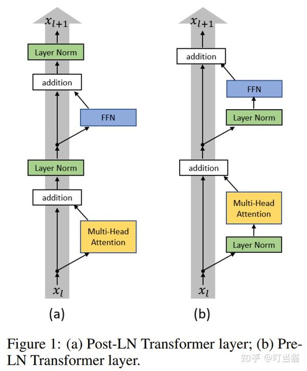
The original "Attention Is All You Need" Transformer architecture used what is now called Post-Layer Normalization (Post-LN). In this configuration, layer normalization is applied after the residual connection.
The operation for a sub-layer (like multi-head attention) is:
Looking at the diagram above (a), you can see that LayerNorm is placed directly on the main information pathway after the "Add" step. While this seems logical, it creates a significant problem: the LayerNorm operation disrupts the clean, identity path for gradients.
As a result, the gradients flowing out of the network's final layers can be very large at the beginning of training, while gradients reaching the initial layers can vanish. This instability forces a workaround. To understand it, please watch the next short video segment.
PostLN, PreLN and ResiDual Transformers
This video from Machine Learning Studio explains the specific issues caused by the Post-LN architecture and the practical 'hack' needed to make it work.
Watch from 01:48 to 03:23. The video explains why Post-LN requires a 'warm-up' stage to prevent training from becoming unstable.
This need for a learning rate warm-up—starting with a tiny learning rate and gradually increasing it—was a major practical challenge. It slowed down training and added sensitive hyperparameters that needed careful tuning. For a long time, the theoretical reason for this was unclear. The paper "On Layer Normalization in the Transformer Architecture" was the first to provide a rigorous explanation.
On Layer Normalization in the Transformer Architecture
Let's read a key section from the paper that formally identified and analyzed this problem.
Please read the section titled 'The Warm-up Problem in Transformer Training'. Focus on the practical challenges that the warm-up requirement creates.
In summary, while Post-LN can achieve high performance, its training is brittle, especially as models get deeper. The gradient flow is unstable, necessitating careful tuning and the inefficient warm-up stage.
3. Pre-Layer Normalization (Pre-LN): The Stable Solution
The solution is remarkably simple: move the normalization layer. In a Pre-Layer Normalization (Pre-LN) architecture, LayerNorm is applied to the input of the sub-layer, before the residual connection.
The operation becomes:
As you can see in diagram (b) above, this change leaves the residual path completely untouched. It creates an uninterrupted highway for gradients to flow from the output all the way back to the input.
Let's see how this simple change fixes the training instability.
PostLN, PreLN and ResiDual Transformers
The same video from Machine Learning Studio now introduces the Pre-LN architecture as the solution.
Watch the brief segment from 03:23 to 03:53. It shows how placing LayerNorm inside the residual block facilitates free gradient flow.
The theoretical analysis in the paper you read from earlier confirms this. It shows that in Pre-LN models, the expected gradient magnitude at initialization naturally shrinks as the model depth () increases, scaling as . This prevents gradients from exploding and makes training stable from the very beginning, eliminating the need for a warm-up.
This stability is why Pre-LN has become the standard for most modern LLMs, including GPT-3 and LLaMA.
4. A Direct Comparison: Stability vs. Performance
We now have two configurations with a clear trade-off. Let's summarize and compare them directly.
| Factor | Post-Norm (Original) | Pre-Norm (Modern) |
|---|---|---|
| Formula | LayerNorm(x + Sublayer(x)) |
x + Sublayer(LayerNorm(x)) |
| Stability | Unstable, especially in deep models. Gradients can explode. | Very stable. Gradients are well-behaved. |
| Warm-up | Required. Training diverges without it. | Not required. Can train with large learning rates from the start. |
| Convergence | Slower, due to the warm-up phase. | Faster, as optimal learning rates can be used earlier. |
| Performance | Can potentially achieve slightly higher final performance. | Very strong performance, but may sometimes regularize too much. |
The following article provides a concise and practical summary of these trade-offs.
Pre-Norm vs Post-Norm: Which to Use?
This article, 'Pre-Norm vs Post-Norm: Which to Use?', gives a great practical overview of the decision-making process.
Please read the following parts: The 'Quick Comparison' table for an at-a-glance summary. The 'How Pre-Norm Works' and 'Why Pre-Norm Stands Out' sections. The 'How Post-Norm Works' and 'Drawbacks and Best Use Cases' sections. The 'Model Size and Depth Considerations' section for practical guidance.
The core trade-off is this: Pre-LN prioritizes training stability, while Post-LN prioritizes representational expressiveness. By normalizing the input to the residual stream, Post-LN can sometimes learn slightly more powerful representations. However, the difficulty of training often outweighs this small potential benefit, especially for the very deep models common today. This has led to the widespread adoption of the more robust Pre-LN architecture.
Conclusion
In this lesson, we've examined the critical architectural choice of placing layer normalization within a Transformer block.
Key Takeaways:
- Residual connections are essential for training deep networks by providing a "shortcut" for gradient and information flow.
- Post-LN, the original design, applies normalization after the residual addition. This disrupts the gradient path, leading to training instability and the need for a learning rate warm-up.
- Pre-LN applies normalization before the sub-layer transformation, leaving the residual path untouched. This ensures stable gradient flow, allowing for faster and more robust training without a warm-up.
- The primary trade-off is stability (Pre-LN) versus potential peak performance (Post-LN). For most modern, very deep LLMs, the stability and efficiency of Pre-LN make it the superior and standard choice.
Preview of the Next Module:
This lesson concludes our module on the modern Transformer stack. We now have a complete picture of how RMSNorm, SwiGLU, RoPE, and Pre-LN come together to form the efficient and stable Transformer block used in today's state-of-the-art models.
In the next module, "Efficient Attention: From MHA to MLA," we'll confront one of the biggest scaling challenges: the computational and memory cost of the attention mechanism itself. Our first lesson will focus on the KV Cache, quantifying its memory demands during text generation and introducing Grouped-Query Attention (GQA) as a first step towards making attention more efficient.