Softmax for Probability Distributions

Introduction

In our last lesson, we established the core principle of autoregressive language modeling: a model like GPT works by repeatedly predicting the next token in a sequence, given all the tokens that came before it. We concluded that the model's fundamental task is to output a probability distribution over its entire vocabulary, indicating how likely each word is to be the next one.

However, a neural network's final layer produces raw, unconstrained numerical scores called logits. These scores might look something like [3.2, -1.5, 0.8, 5.1, ...], where each number corresponds to a token in the vocabulary. The larger the number, the more the model "favors" that token. But these are not probabilities—they aren't between 0 and 1, and they don't sum to 1.

This lesson bridges that gap. We will explore the softmax function, the mathematical tool used in virtually all classification and language models to transform raw logits into a clean, interpretable probability distribution.

By the end of this lesson, you will be able to:

• Explain the purpose of the softmax function.
• Compute the softmax function for a given vector of logits.
• Understand a key practical issue: numerical stability.
• Describe how the "temperature" parameter affects the output distribution.

From Logits to Probabilities: The Softmax Function

The challenge is to convert a vector of arbitrary real numbers (logits) into a probability distribution. This distribution must have three key properties:

1. All output values must be in the range [0, 1].
2. The sum of all output values must be exactly 1.
3. The transformation should preserve the order of the original scores (a higher logit should result in a higher probability), and ideally, it should amplify the model's confidence in its top choice.

The softmax function achieves this through a two-step process:

1. Exponentiation: To ensure all outputs are positive and to amplify the larger logit values, we apply the exponential function ($e^x$) to each logit.
2. Normalization: To make the values sum to 1, we divide each exponentiated logit by the sum of all exponentiated logits.

The Mathematical Definition

For an input vector of logits $\mathbf{z}=[z_1,z_2,\dots ,z_K]$, where $K$ is the size of the vocabulary, the softmax function $\sigma (\mathbf{z})$ produces an output vector where the $i$-th element is calculated as:

$\sigma (\mathbf{z}{)}_i=\frac{e^{z_i}}{{\sum }_{j=1}^K{e}^{z_j}}$

This process is visualized clearly in the following diagram.

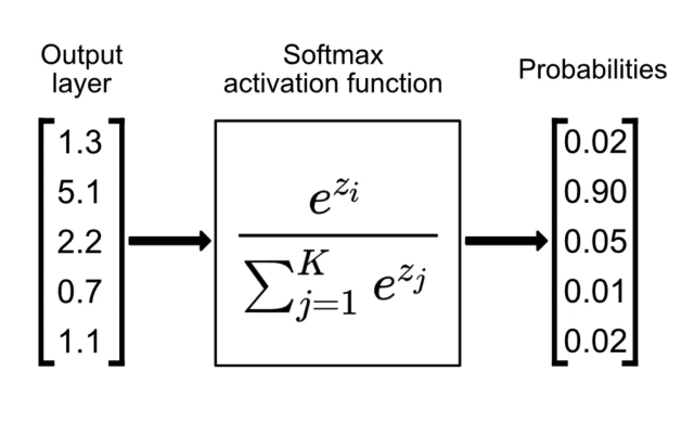
You might recognize this as a similar setup to the final layer of a Convolutional Neural Network (CNN) used for multi-class image classification. The principle is identical: converting raw class scores into class probabilities.

A Step-by-Step Example

Let's compute this for a small example. Imagine a language model with a vocabulary of just four words, and for a given input, it produces the logits: [1.2, 0.3, -0.5, 2.8].

The following resource provides an excellent walkthrough of the computation, which we will follow here.

Following the steps from the article:

1. Get Raw Scores (Logits):
   z = [1.2, 0.3, -0.5, 2.8]

2. Apply the Exponential:

   • $e^{1.2}\approx 3.320$
   • $e^{0.3}\approx 1.350$
   • $e^{-0.5}\approx 0.607$
   • $e^{2.8}\approx 16.445$

3. Sum All Exponentials:
   3.320 + 1.350 + 0.607 + 16.445 = 21.722

4. Divide Each by the Sum (Normalize):

   • Prob(Word 1): $3.320/21.722\approx 0.153$ (15.3%)
   • Prob(Word 2): $1.350/21.722\approx 0.062$ (6.2%)
   • Prob(Word 3): $0.607/21.722\approx 0.028$ (2.8%)
   • Prob(Word 4): $16.445/21.722\approx 0.757$ (75.7%)

The final probability distribution is [0.153, 0.062, 0.028, 0.757]. The model is now telling us it is 75.7% confident that the fourth word in the vocabulary is the correct next token.

A Practical Imperative: Numerical Stability

What happens if the logits are large? For example, if your logits are [990, 1000, 995]. Computing $e^{1000}$ would result in a number so massive that it causes a numerical overflow in standard floating-point arithmetic.

To solve this, a clever trick is used in all production-level implementations. The following resource explains this essential technique.

As the article explains, you can subtract any constant from all logits before applying softmax, and the final probabilities will be identical. By choosing to subtract the maximum logit value, you ensure that the largest input to the exponential function is 0 ($e^0=1$), and all other inputs are negative. This prevents overflow while producing the exact same result.

The stable softmax is computed as:
$\sigma (\mathbf{z}{)}_i=\frac{e^{z_i-\max (\mathbf{z})}}{{\sum }_{j=1}^K{e}^{z_j-\max (\mathbf{z})}}$

Deeper Intuition: Temperature and Geometry

Now that you understand the mechanics, let's build a deeper, more visual intuition for what softmax is doing. The following videos explore the geometry of the function and introduce an important hyperparameter called temperature.

First, let's see how softmax converts logits into probabilities and the properties that arise from its mathematical form.

The temperature parameter is especially important in language models. By dividing the logits by a temperature value $T$ before applying the softmax, we can control the randomness of the model's predictions during generation.
$\sigma (\mathbf{z},T{)}_i=\frac{e^{z_i/T}}{{\sum }_{j=1}^K{e}^{z_j/T}}$

• $T>1$ (higher temperature) "softens" the probability distribution, making it more uniform. This increases randomness, leading to more creative or diverse outputs.
• $T<1$ (lower temperature) "sharpens" the distribution, making the model more confident in its top choice. This reduces randomness, leading to more deterministic and focused outputs.
• $T=1$ is the standard softmax.

This next video offers a concise explanation of why we need softmax and how temperature scaling helps correct for the overconfidence that the exponential function can introduce.

Conclusion

In this lesson, we demystified a critical component of modern neural networks. You now understand how a language model can produce a coherent probability distribution from the raw scores it generates.

Key Takeaways:

• The softmax function transforms a vector of raw scores (logits) into a probability distribution.
• It operates in two steps: exponentiating each logit to make it positive, and then normalizing by dividing by the sum of all exponentiated values.
• A crucial implementation detail is the numerical stability trick: subtracting the maximum logit from all logits before exponentiation to prevent overflow. This does not change the final probabilities.
• The temperature parameter ($T$) is a powerful tool used during generation to control the sharpness of the output distribution, balancing between deterministic and random sampling.

Preview of the Next Lesson:

Now that we have a probability distribution for the next token (e.g., [0.15, 0.06, 0.03, 0.76]), how do we use this to train the model? We need a way to compare this predicted distribution to the actual next token from the training data and calculate a single number representing the error or "loss."

In the next lesson, we will introduce the cross-entropy loss function, which is the standard method for measuring this error and providing the gradient signal that drives the entire learning process.