KV Cache: Efficient Autoregressive Inference

Introduction

In our previous lesson, we demystified the autoregressive process, seeing how decoder-only models generate text one token at a time in a predict -> sample -> append loop. We concluded by highlighting a significant inefficiency: at every step, the model re-processes the entire sequence from the beginning. For a 100-token prompt and a 100-token generation, this involves an enormous amount of redundant computation.

This lesson tackles that problem head-on. Our learning outcome is to explain the KV cache mechanism and how it avoids redundant computation during autoregressive inference. The KV cache is not an approximation; it is a fundamental optimization that makes the fast, interactive experience of modern LLMs possible. By the end of this lesson, you will understand what the KV cache is, why it works, and how it transforms the computational complexity of text generation from quadratic to linear.

1. The Redundancy Problem in Autoregressive Generation

To understand the solution, we must first pinpoint the exact source of the waste. Recall that in the attention mechanism, each token's input embedding is projected into three vectors: a Query (Q), a Key (K), and a Value (V).

• Query: "What am I looking for?"
• Key: "What information do I contain?"
• Value: "What information I will provide if attended to?"

The critical insight is that for any given token in the input sequence, its Key and Value vectors are always the same. They are computed by multiplying the token's embedding by the fixed projection matrices $W_K$ and $W_V$. No matter how many new tokens are generated afterwards, the Key and Value for "The" in "The cat sat on the mat" will never change.

However, in the naive generation loop, we recompute them at every single step.

To build a strong intuition for this problem, let's start with a conceptual overview.

As the article illustrates, the attention mechanism is constantly re-running the same calculations on the initial prompt tokens. Now, let's get a more formal look at where this happens in the attention formula.

2. The KV Cache Solution: Compute Once, Reuse Often

The solution is as elegant as the problem is clear: if the Key and Value vectors for past tokens don't change, we should compute them once and store them. This is the essence of the KV cache.

The generation process is split into two phases:

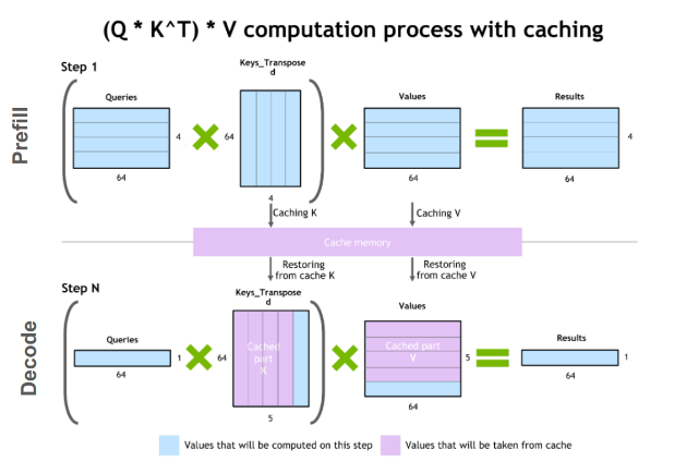
1. Prefill: The model processes the entire input prompt at once. It computes the K and V vectors for all prompt tokens and saves them in the cache.
2. Decode: For each subsequent step, the model only needs to perform computations for the single new token. It computes the new token's Q, K, and V vectors. It then appends the new K and V to the cache. Finally, it uses the new token's Q vector to attend to all the K and V vectors stored in the cache (from the prompt and all previously generated tokens).

This creates an important asymmetry:

• Keys and Values are cached because they represent the static properties of tokens already in the sequence.
• Queries are not cached because a query is always "new" for the token being generated, asking how it should relate to all the history that came before it.

The following image provides a clear visual summary of this two-phase process.

To further solidify this, the following video provides a helpful analogy.

3. Cache Structure and Mathematical Formulation

Since you appreciate the underlying math, let's formalize this. With a KV cache, the computation at each decode step t becomes much simpler. We only compute the projections for the single new token's embedding, $x_t$:

We then append the new key ($k_t$) and value ($v_t$) vectors to our cache:

The attention output for the new token, $o_t$, is then computed using the new query $q_t$ and the entire history stored in the cache:

This is not an approximation; it's an algebraically equivalent way to get the exact same result as the naive method, but with drastically fewer computations.

This cache must be maintained for each attention head and for each layer of the Transformer, as they all learn unique projection matrices.

For a deeper dive into the mathematical details and the cache's structure, the "KV Cache Explained" article is an excellent resource.

4. Implementation and Performance Impact

Seeing this in code makes the concept even more concrete. The implementation involves adding buffers to store the cache and a flag to switch between the initial prefill and the subsequent decode steps.

The core change is in the generation loop. Without a cache, you feed the entire sequence model(idx) at each step. With a cache, you do one prefill model(idx, use_cache=True), and then feed only the single next_idx in the decode loop: model(next_idx, use_cache=True).

This change from quadratic to linear complexity has a massive impact on inference speed. The Welch Labs video provides a striking example of the KV cache's memory footprint, which is the trade-off for this speed.

As the video shows, while the computational savings are huge, the memory required to store the cache for long sequences can become a new bottleneck—a problem that advanced architectures like DeepSeek's MLA (which we will study later) are designed to solve.

Conclusion

In this lesson, we have explored the KV cache, a simple yet profoundly important optimization for LLM inference.

Key Takeaways:

• The Problem: Naive autoregressive generation is inefficient because it repeatedly recomputes Key and Value vectors for tokens that have not changed, leading to quadratic computational complexity.
• The Solution: The KV cache stores these Key and Value vectors after they are computed once. In subsequent steps, the model only computes projections for the new token and reuses the cached values.
• The Impact: This changes the computational complexity of generation from quadratic, $O(T^2)$, to linear, $O(T)$, with respect to the sequence length $T$.
• The Trade-off: The speed-up comes at the cost of memory. The cache size grows linearly with the sequence length and can become substantial for large models and long contexts.
• Structure: The cache is maintained on a per-layer, per-head basis, as each of these components learns independent K and V projections.

Preview of the Next Lesson:
We have now completed our foundational module on Transformer architecture basics. We've seen how tokens become vectors, how attention creates context, and how autoregressive generation with the KV cache produces text efficiently.

Next, we will begin our deep dive into the Modern Transformer Components that define state-of-the-art models. Our first lesson in this new module will explore RMSNorm and the SwiGLU activation function, two key architectural tweaks that improve training stability and model performance, moving us closer to understanding the design of models like Qwen 2.5 and DeepSeek-V3.