Understanding LayerNorm for Stable Training

Introduction

In our last lesson, we assembled the complete Transformer block, identifying its four essential components: the self-attention layer, the feed-forward network (FFN), residual connections, and layer normalization. We briefly touched on the "Add & Norm" steps that are crucial for enabling deep networks.

Today, we're going to zoom in on the "Norm" part of that step. Our learning outcome is to explain LayerNorm and how it stabilizes training in deep networks. We will dissect this technique from first principles, understanding the problem it solves, its mathematical formulation, and why it is the standard choice for Transformers. This deep dive will clarify exactly how LayerNorm prevents the training process from becoming unstable, a critical piece of knowledge for understanding how massive models like GPT can be trained at all.

1. The Problem: Why Deep Networks are Unstable

As we stack more and more Transformer blocks to create a deep network, a fundamental problem arises: training becomes unstable. The output of one layer is the input to the next. Small changes in the weights of early layers can cause the distribution of activations (the outputs of each layer) in later layers to shift dramatically during training. This phenomenon is often called internal covariate shift.

This "activation scale drift" leads to two nightmares for training:

1. Exploding Gradients: If activations multiply and grow exponentially through the layers, they can become enormous. The resulting gradients calculated during backpropagation will also be enormous, causing weight updates to be so large that the model's parameters "explode" towards infinity. The loss becomes NaN (Not a Number), and training collapses.
2. Vanishing Gradients: Conversely, if activations repeatedly shrink, they can become vanishingly small. The gradients then approach zero, meaning the model's weights stop updating, and learning grinds to a halt.

To build intuition, let's explore an article that frames this problem clearly.

The core idea of normalization is to counteract this drift by rescaling the activations at every layer, ensuring they have a predictable and stable distribution before being passed on.

2. Normalization: Batch vs. Layer

A common normalization technique you might have encountered in the context of CNNs is Batch Normalization (BatchNorm). BatchNorm normalizes activations by computing the mean and variance for each feature across the entire batch of training examples.

However, this approach is ill-suited for sequence models like Transformers. Why?

• Variable Sequence Lengths: Sentences in a batch have different lengths. Forcing them into a fixed-size tensor requires padding, and calculating statistics over a mix of real tokens and padding tokens is problematic.
• Incoherent Batch Statistics: A token at position 5 in one sentence has no semantic relationship to the token at position 5 in another. Calculating a batch-wide mean for "position 5" is statistically meaningless.

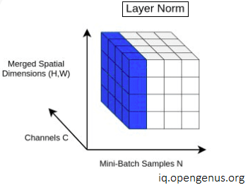
Layer Normalization (LayerNorm) solves this by changing the axis of normalization. Instead of normalizing across the batch, it normalizes across the features for each token independently.

This independence from the batch is LayerNorm's superpower for Transformers. It doesn't matter how long the sequence is or what other sequences are in the batch; each token's activation vector is treated as a self-contained unit to be normalized.

Let's read a short piece that makes this distinction crystal clear.

3. A Mathematical Deep Dive into LayerNorm

Now, let's break down the LayerNorm formula step-by-step. For a given token, its activation is a vector $\mathbf{x}$ with $d$ dimensions (e.g., $d=768$). The goal is to transform this vector so its elements have a mean of 0 and a variance of 1.

The following resource provides an excellent, detailed walkthrough of the math. We'll use it as our guide.

Let's summarize the key steps from the reading:

Step-by-Step Breakdown:

1. Calculate the Mean ($\mu$): First, we find the average value of all the features for a single token's activation vector $\mathbf{x}$.
   $\mu =\frac{1}{d}{\sum }_{i=1}^d{x}_i$

2. Calculate the Variance (${\sigma }^2$): Next, we measure how spread out the features are from this mean.
   ${\sigma }^2=\frac{1}{d}{\sum }_{i=1}^d(x_i-\mu {)}^2$

3. Normalize: We use the mean and standard deviation ($\sigma =\sqrt{{\sigma }^2}$) to standardize each feature $x_i$, shifting its mean to 0 and scaling its variance to 1.
   ${\hat{x}}_i=\frac{x_i-\mu }{\sqrt{{\sigma }^2+ϵ}}$
   The $ϵ$ (epsilon) is a very small number (e.g., $10^{-5}$) added for numerical stability to prevent division by zero if the variance is zero.

4. Scale and Shift: Forcing every layer's activations to have a mean of 0 and variance of 1 can be too restrictive. The network might lose representational power. To solve this, LayerNorm introduces two learnable parameter vectors, gamma ($\gamma$) and beta ($\beta$), each of dimension $d$. These are initialized to 1s and 0s, respectively.
   $y_i={\gamma }_i\cdot {\hat{x}}_i+{\beta }_i$
   This final step allows the network to learn the optimal scale and shift for each feature dimension. If the network finds it beneficial, it can learn to effectively "undo" the normalization by setting $\gamma$ and $\beta$ appropriately. This means LayerNorm stabilizes training without reducing the model's capacity.

Putting it all together, the full formula for a vector $\mathbf{x}$ is:
$\text{LayerNorm}(\mathbf{x})=\gamma \odot \frac{\mathbf{x}-\mu }{\sqrt{{\sigma }^2+ϵ}}+\beta$
where $\odot$ denotes element-wise multiplication.

4. LayerNorm in Practice

Let's see how this translates to code. Your familiarity with PyTorch will make this straightforward. The code mirrors the mathematical steps we just covered.

The key takeaways from the practical implementation are:

• The mean and variance are computed over the last dimension (dim=-1), which is the feature dimension in a typical (batch, sequence, features) tensor.
• The learnable gamma and beta parameters correspond to weight and bias in PyTorch's nn.LayerNorm module.
• The transformation successfully reshapes a feature distribution with an arbitrary mean and standard deviation to one that is tightly controlled, with a mean of ~0 and a standard deviation of ~1 (before applying gamma and beta).

Conclusion

In this lesson, we took a comprehensive look at Layer Normalization, a cornerstone of the Transformer architecture.

Key Takeaways:

• Problem: Deep neural networks suffer from unstable training due to internal covariate shift, which can lead to exploding or vanishing gradients.
• Solution: Layer Normalization stabilizes training by normalizing the activations at each layer.
• Mechanism: For each token's activation vector, LayerNorm computes the mean and variance across the feature dimension and uses them to scale the vector to have a mean of 0 and a standard deviation of 1.
• Flexibility: Learnable scale ($\gamma$) and shift ($\beta$) parameters are applied after normalization, allowing the network to learn the optimal distribution for its features, thus preserving representational power.
• Suitability for Transformers: Because it operates on each sample independently, LayerNorm works perfectly with the variable sequence lengths and batch sizes common in NLP.

Preview of the Next Lesson:
We have now fully dissected the components of a standard Transformer block. These blocks are used in both encoder-only models (like BERT), decoder-only models (like GPT), and encoder-decoder models (the original Transformer). In our next lesson, we will distinguish between these different high-level architectures and understand their typical use cases, setting the stage for understanding modern LLMs, which are predominantly decoder-only.