Greedy Search for Approximate Nearest Neighbor

The Core Idea: Greedy Routing

The fundamental principle behind searching a Navigable Small World graph is remarkably simple and elegant. We want to find the node in the graph whose vector is closest to a given query vector. Instead of checking every single node, we perform a guided traversal.

The process, known as greedy search or greedy routing, works like this:

1. Start at a designated entry point in the graph.
2. At your current node, examine all of its immediate neighbors.
3. Calculate the distance from each neighbor to the query vector.
4. Move to the neighbor that is closest to the query.
5. Repeat steps 2-4 until you reach a node where none of its neighbors are closer to the query than the node itself. This node is a local minimum with respect to the query, and it is our approximate nearest neighbor.

This simple, local decision-making process allows for an efficient traversal of the graph. The combination of short-range and long-range links we discussed previously ensures that these local decisions can quickly guide the search across the vector space.

The "Local Minimum" Problem

While simple greedy search is fast, it has a significant weakness: it can get stuck. The algorithm's "myopic" nature—always moving to the closest immediate neighbor—means it will never make a move that temporarily increases the distance to the query, even if that move is necessary to find a better long-term path.

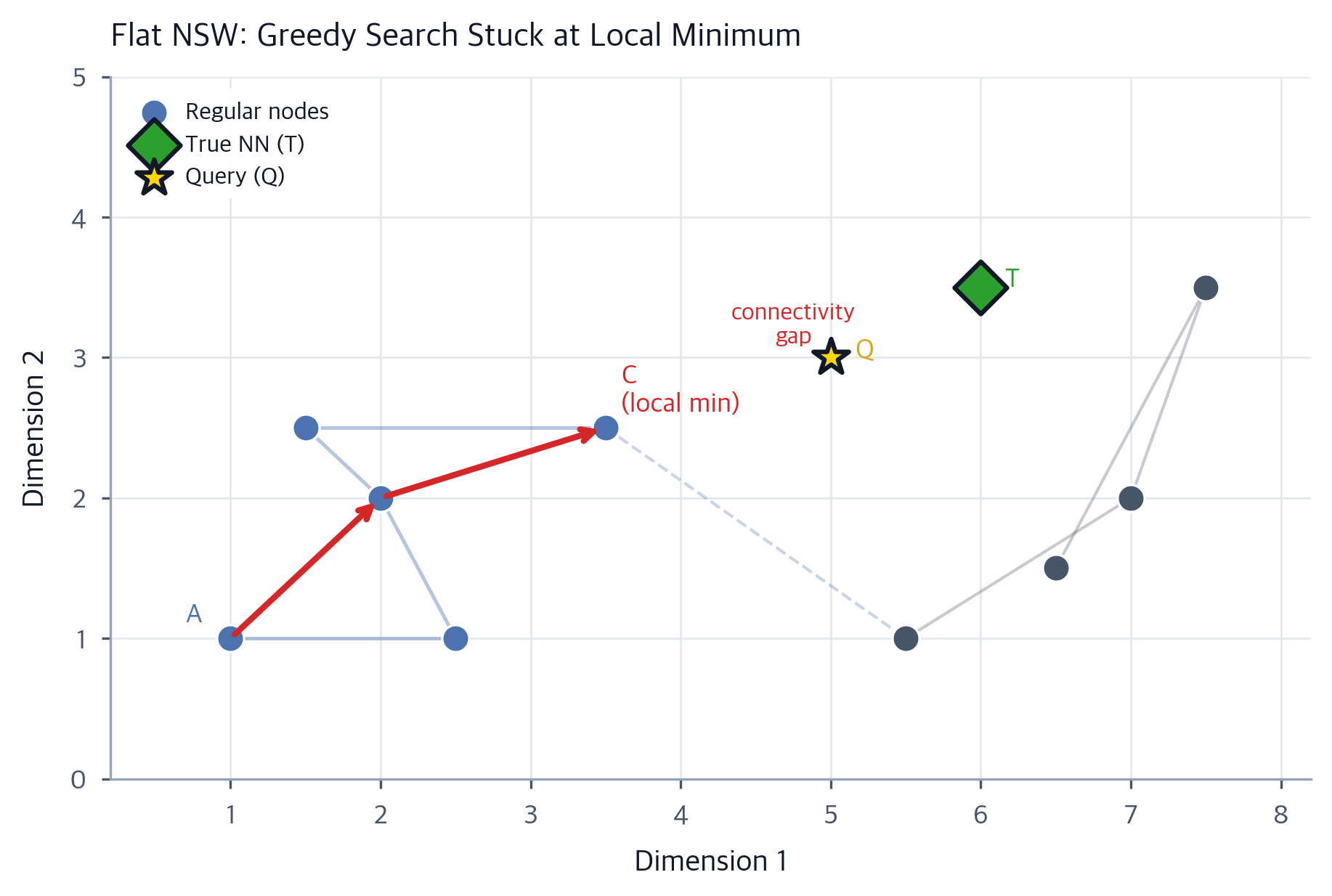
This is the classic "local minimum" problem. The search has found a point that is a minimum within its immediate neighborhood, but it is not the global minimum for the entire graph.

To build a robust search system, we need an algorithm that is less susceptible to this problem.

A More Robust Algorithm: Beam Search

The solution is to be less greedy. Instead of tracking only the single best candidate at each step, we can maintain a list of several good candidates. This technique is a form of beam search. It allows the algorithm to explore multiple paths simultaneously, dramatically reducing the chance of getting permanently stuck in a suboptimal region of the graph.

The standard HNSW paper formalizes this robust greedy search in an algorithm called SEARCH-LAYER. This is the algorithm we will implement. It maintains three key data structures:

• v (visited set): A set of node indices that have already been considered. This prevents us from getting into infinite loops and doing redundant work. In our C implementation, a simple bool array or a more memory-efficient bitset is ideal.
• C (candidates): A priority queue of nodes to visit, ordered by their distance to the query (closest first). This is our "beam."
• W (results): A priority queue containing the best ef nodes found so far, ordered by their distance to thequery (farthest first). This allows us to quickly identify the worst node in our current result set.

The ef parameter (for "effective search") is crucial here. It defines the size of the candidate and result lists, essentially the "width" of our search beam. A larger ef value makes the search more thorough and accurate, at the cost of more distance computations. This is a direct, tunable tradeoff between speed and recall, a concept central to performance systems engineering.

Let's break down the logic of SEARCH-LAYER:

1. Initialization: The visited, candidates, and results sets are all initialized with the entry point(s).
2. Main Loop: The loop continues as long as there are candidates in C.
3. Extract Best Candidate: In each iteration, remove the node c from C that is closest to the query q.
4. Termination Check: This is the most clever part of the algorithm. Compare the distance of c to the query with the distance of the farthest node f in our result set W. If distance(c, q) > distance(f, q), it means that the best candidate we have left to explore is already worse than the worst result we have found so far. No further exploration from this path can improve our result set, so we can terminate the search early.
5. Neighbor Exploration: For each neighbor e of the current node c:
   • If e has not been visited, mark it as visited.
   • If distance(e, q) is less than the distance of the farthest node in W, or if W isn't full yet, then e is a good candidate. Add it to C and W.
   • If W is now larger than ef, remove the farthest element to maintain its size.
6. Return: Once the loop terminates, W contains the ef nearest neighbors found during the search.

This SEARCH-LAYER algorithm is the workhorse of both search and insertion in HNSW. While our full project will use it across multiple hierarchical layers, for this lesson, we will implement it to run on our single-layer NSW graph.

Implementation in C

Now, let's translate this into a C function. Based on the previous lesson, you should be comfortable with a bounded max-heap for managing the top 'k' candidates. We'll use that concept for our candidates and results lists.

A plausible function signature would look like this:

#include <stdbool.h>
#include <stdint.h>

// Forward declaration from our previous lesson's data structures
typedef struct HNSWGraph HNSWGraph;

// A struct to hold a single search result
typedef struct {
    uint32_t index; // Index of the node in the graph's node pool
    float distance; // Distance to the query vector
} SearchResult;

/**
 * @brief Performs a greedy search on a single layer of the graph.
 * 
 * @param graph A pointer to the initialized HNSWGraph.
 * @param query_vector The vector we are searching for.
 * @param entry_point_index The index of the node to start the search from.
 * @param ef_search The size of the dynamic candidate list (beam width).
 * @param k The number of nearest neighbors to return.
 * @param results An output array to store the top k results.
 * @return The number of neighbors found (up to k).
 */
int nsw_search(
    const HNSWGraph* graph, 
    const float* query_vector,
    uint32_t entry_point_index,
    int ef_search,
    int k,
    SearchResult* results
);

Inside this function, you will need to manage the three data structures:

• Visited Set: A bool visited[graph->capacity] array is simple and effective. Initialize it to all false.
• Candidates (C): A min-heap data structure to efficiently retrieve the closest candidate.
• Results (W): A max-heap data structure to efficiently find and remove the farthest result.

Since you've already implemented a bounded max-heap, you can adapt that logic. The main challenge is managing two heaps and the visited set in accordance with the SEARCH-LAYER algorithm's logic. Your task is to implement the body of this nsw_search function.

Conclusion

In this lesson, we've dissected the core search algorithm that powers our vector database. We moved from a simple, intuitive greedy search to a robust beam search that avoids the common pitfalls of local minima.

Key Takeaways:

• Greedy Search: A fast, simple graph traversal strategy that always moves to the neighbor closest to the query.
• Local Minima: The primary weakness of a simple greedy search, where it can get trapped in a suboptimal region of the graph.
• Beam Search (SEARCH-LAYER): A more robust algorithm that maintains a "beam" of ef candidates, allowing it to explore multiple paths and find better results.
• Performance Tradeoff: The ef_search parameter provides a direct way to tune the balance between search speed and accuracy (recall), a critical feature for any high-performance search system.
• Core Logic: The algorithm's efficiency stems from its early termination condition: the search stops once the best available candidate is worse than the worst result already found.

You now have the "map" (our data structures from the last lesson) and the "GPS" (the search algorithm). In our next lesson, we will put them together to tackle the problem of graph construction. You'll see that the nsw_search function you are building now is not only used for querying but is also a critical subroutine for inserting new vectors into the graph.