Graph Data Structures in C

The Primacy of Data Locality

Before we write a single line of a struct, we must understand why its design is so critical for performance. In modern computing, there's a vast and ever-widening performance gap between the CPU and main memory (RAM). A CPU can perform calculations in a few cycles, but fetching data from RAM can take hundreds. To bridge this gap, CPUs use small, fast caches.

When the CPU needs to read a byte from memory, it doesn't just fetch that single byte. It fetches an entire cache line—a contiguous block of memory, typically 64 bytes. If the next piece of data the CPU needs is already in that cache line, it's a cache hit, which is extremely fast. If it's not, it's a cache miss, forcing a slow trip to main memory.

Our mission, as performance engineers, is to maximize cache hits. The key to this is data locality: arranging data that is accessed together, close together in memory.

If we were to allocate each node of our graph using a separate call to malloc, the memory manager could place them anywhere in the heap. Traversing the graph would mean jumping unpredictably across memory—a pattern known as "pointer chasing"—which is devastating for cache performance. We must do better.

Designing the Graph Structs

Let's start designing our data structures with data locality as our guiding principle. An NSW graph consists of nodes (our vectors) and edges (connections between them).

A common object-oriented approach might be:

// Naive approach - DO NOT USE
struct Node {
    float* vector;
    struct Node** neighbors; // A dynamic array of pointers to neighbors
    int neighbor_count;
};

This seems reasonable, but it's a performance trap. The neighbors array contains pointers. Following each pointer during a search is a potential cache miss. We are scattering our data accesses all over memory.

A much better approach is to store everything in large, contiguous arrays and use simple integer indices instead of pointers to represent relationships.

Consider a Graph struct that owns all the memory:

// A better, data-oriented design
typedef struct {
    // Memory pool for all nodes
    HNSWNode* nodes;
    // Memory pool for all vectors
    float* vectors;

    // Metadata
    size_t capacity;       // Max number of nodes we can store
    size_t count;          // Current number of nodes in the graph
    size_t vector_dim;     // The dimension of each vector
    // ... other graph-wide parameters ...
} HNSWGraph;

Here, all nodes will live in a single block of memory pointed to by nodes, and all vector data will live in another block pointed to by vectors. This is our contiguous memory pool.

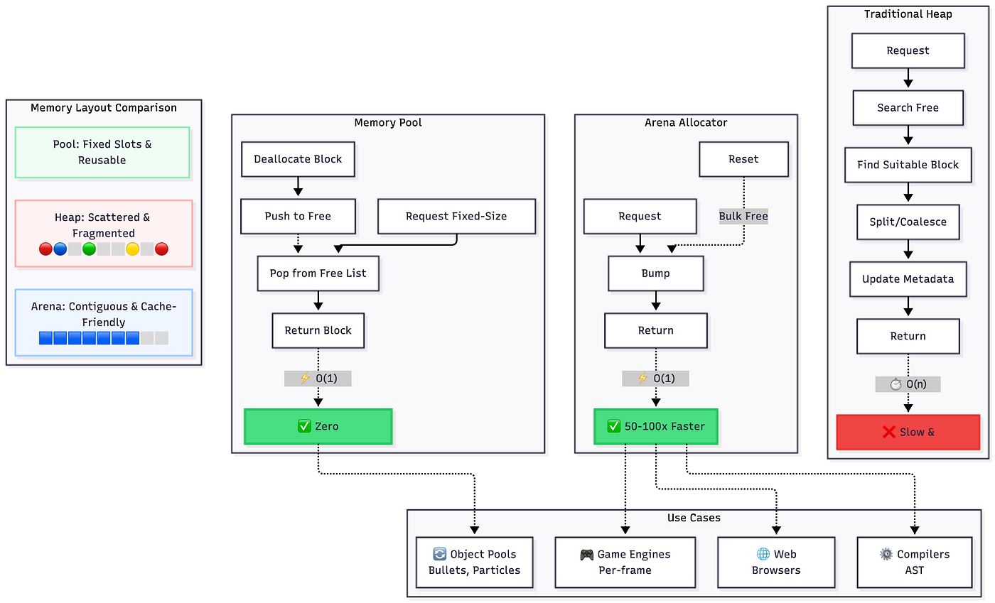
This diagram compares the traditional heap against memory pools and arenas. Our approach is a form of Arena Allocator, where we pre-allocate a large memory region and serve allocation requests from it, offering significant speed advantages and better data locality.

Now, let's design the HNSWNode struct. What does each node need to know?

1. Where its vector data is.
2. Which other nodes it's connected to.

Instead of pointers, we will use indices. An index i will refer to the i-th node in the nodes array and the i-th vector in the vectors array.

#define MAX_NEIGHBORS 32 // Example: each node can have up to 32 neighbors

typedef struct {
    // The list of neighbors, stored as indices into the main `nodes` array.
    uint32_t neighbors[MAX_NEIGHBORS];
    
    // The number of valid neighbors currently in the `neighbors` array.
    uint8_t neighbor_count;

    // We can add other per-node data here as needed.
    // For example, the `antirez` HNSW implementation uses an 'epoch'
    // system to efficiently track visited nodes during a search.
    // uint64_t visited_epoch;
    
} HNSWNode;

Notice a few key decisions here:

• No separate Edge struct: An edge is simply the relationship between two nodes. We represent it implicitly by storing one node's index in another's neighbors array. This is highly efficient.
• Indices, not pointers: neighbors is an array of uint32_t, not HNSWNode*. A 32-bit index can address up to 4 billion nodes, which is plenty for many use cases, and it's half the size of a 64-bit pointer. This makes our HNSWNode struct smaller, meaning more nodes can fit into a single cache line.
• Fixed-size neighbor array: We've pre-allocated space for MAX_NEIGHBORS. This simplifies memory management immensely. We don't need to realloc anything when adding a neighbor (up to the limit). This is a common tradeoff in high-performance computing: sacrificing some flexibility for predictable, fast performance.

This design is analogous to the adjacency list representation of a graph, but optimized for cache-friendliness.

This image shows a graph represented by a Vertex array and an Edge array. Our design is similar: the nodes pool is our vertex array, and the neighbors array inside each node struct serves as a distributed version of the edge array, keeping edge information local to each vertex.

The Memory Pool in Practice

With this design, allocating a new node becomes trivial. We aren't calling malloc. We simply use the next available slot in our pre-allocated nodes array.

1. The HNSWGraph is initialized, allocating a large chunk of memory for nodes and vectors based on its capacity.
2. When we insert the first vector, its data is copied to vectors[0] and its node is initialized at nodes[0]. The graph's count becomes 1.
3. The second vector goes into vectors[1], its node at nodes[1], and count becomes 2.
4. And so on. Allocation is just graph->count++. This is an O(1) operation, orders of magnitude faster than a typical malloc call.

This strategy is often called a "Pool Allocator" or an "Arena Allocator". The video below gives a practical walkthrough of implementing such a system. While it's in C++ and more complex than our simple bump allocator, the core principles of pre-allocation and managing blocks are the same.

By designing our data structures and allocation strategy together, we ensure that as we traverse the graph—hopping from a node to its neighbors—we are likely making sequential or short-range jumps within a single, large block of memory. This is exactly the kind of predictable access pattern that the CPU's prefetcher loves, keeping the caches full and the CPU busy with useful work.

Conclusion

In this lesson, we made the crucial leap from abstract graph theory to concrete, performance-oriented C data structures. We've seen that for high-performance systems, data structure design is inseparable from memory layout design.

Key Takeaways:

• Data Locality is King: The high cost of cache misses means that how we arrange data in memory is as important as the algorithms that process it.
• Avoid Pointer Chasing: We use integer indices instead of raw pointers to represent relationships between nodes, making our structs smaller and data access more direct.
• Contiguous Allocation: All nodes are allocated from a large, pre-allocated memory pool (an arena). This makes allocation extremely fast (O(1)) and maximizes spatial locality, keeping related data physically close in memory.
• Implicit Edges: We don't need a separate Edge struct. Connections are implicitly defined by the neighbors array within each HNSWNode, a design that is both memory-efficient and cache-friendly for traversal.

We have now designed the "map" of our vector world. In the next lesson, we will implement the "GPS" to navigate it. We will write the C code for the greedy search algorithm that traverses this very data structure to find the approximate nearest neighbors for a query vector.