Implementing SEARCH-LAYER for k-NN in a Single Graph Layer

The Search Within a Layer

Imagine the multi-layer HNSW graph. The full search process involves starting at the top layer and "drilling down." The SEARCH-LAYER algorithm is the procedure that executes the horizontal search on each of those flat planes.

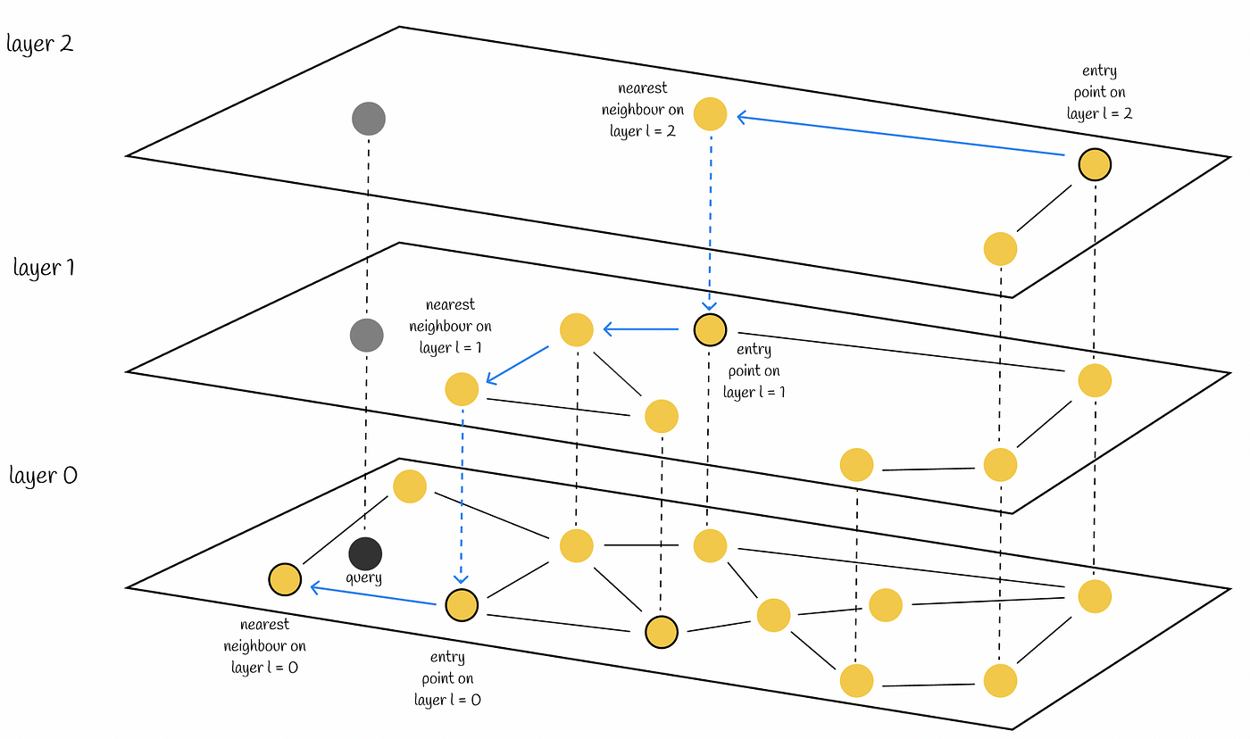
At its core, SEARCH-LAYER is a best-first or greedy search algorithm. Given one or more starting points (entry points), it iteratively explores the graph, always moving toward the nodes that are closest to our query vector.

The following video provides an excellent high-level intuition for this greedy traversal, which the author calls "greedy routing."

While this explains the basic principle, the actual SEARCH-LAYER algorithm is more robust. It doesn't just explore a single path; it maintains a pool of candidates to avoid getting stuck too early in a poor local minimum.

Algorithm 2: The Blueprint for SEARCH-LAYER

The original HNSW paper provides the definitive pseudocode for this procedure in "Algorithm 2." This will be our blueprint for implementation.

Let's dissect this algorithm. It requires three key data structures to manage its state:

1. v (Visited Set): A set to keep track of nodes we have already processed. This prevents us from getting stuck in cycles and doing redundant work. A hash set is a viable option, but for maximum performance, we'll discuss a common systems-level optimization for this shortly.

2. C (Candidates): A collection of candidate nodes to visit, ordered by their distance to the query vector q. The node with the smallest distance should be processed next. This is a perfect use case for a min-priority queue (or min-heap).

3. W (Working Set / Results): A collection of the ef nearest neighbors found so far, ordered by their distance to the query. To efficiently check if a new node is better than the worst node currently in our results, we need to quickly access the element with the largest distance. This calls for a max-priority queue (or max-heap).

The Algorithm Step-by-Step

Let's walk through the logic of SEARCH-LAYER(q, ep, ef, lc):

• Initialization (Lines 1-3):

  • Initialize v, C, and W with the entry point(s) ep. The distances from the entry points to the query q are calculated.
  • v now contains ep.
  • The min-heap C contains ep, prioritized by its distance to q.
  • The max-heap W contains ep, also prioritized by its distance to q.

• Main Loop (Line 4): The search continues as long as there are candidates in C.

• Candidate Selection (Line 5):

  • Extract the best candidate c from the min-heap C. This is the node closest to q that we haven't explored yet.

• Early Termination Condition (Lines 6-8):

  • Get the furthest element f currently in our results W. This is simply a peek at the top of the max-heap.
  • if distance(c, q) > distance(f, q): This is a critical performance optimization. It means the best unexplored candidate (c) is already further away than the worst node in our result set (f). Since all other candidates in C are even further than c (it's a min-heap), we know that no further exploration can improve our result set W. We can safely terminate the search for this layer.

• Neighbor Exploration (Lines 9-17):

  • For each neighbor e of the current node c (on the specified layer lc):
    • If e has not been visited:
      • Mark e as visited.
      • Get the furthest element f from W.
      • if distance(e, q) < distance(f, q) or |W| < ef: This is the condition for adding a neighbor to our sets. We are interested in e if either:
        1. Our result set W is not yet full (i.e., we have found fewer than ef neighbors).
        2. The neighbor e is closer to the query q than the furthest neighbor f in W.
      • If the condition passes, add e to both the candidate min-heap C and the result max-heap W.
      • If adding e makes W exceed the size ef, remove the furthest element from W (i.e., pop from the max-heap).

• Return (Line 18):

  • Return the final set of nearest neighbors, W.

Implementation Notes for High Performance

Your background in systems programming will appreciate that the choice of data structures here is paramount for performance.

• Heaps for C and W: A textbook implementation in C would involve creating a binary heap backed by a dynamic array. You would implement heap_push and heap_pop functions that maintain the heap property. This avoids the overhead of more complex standard library containers. For C, it's a min-heap; for W, a max-heap.

• The "Visited" Set (v): A hash set can have non-trivial overhead (hashing, memory allocations). A far more efficient technique used in production systems is the epoch trick.

  1. Add a global uint64_t search_epoch; counter to your main HNSW index struct.
  2. Add a uint64_t visited_epoch; field to your hnswNode struct.
  3. When a new search starts (the top-level k-NN-SEARCH call, not SEARCH-LAYER), increment the global search_epoch.
  4. To "mark a node as visited" within SEARCH-LAYER, you set node->visited_epoch = global_search_epoch;.
  5. To "check if visited," you simply compare node->visited_epoch == global_search_epoch;.

  This approach is incredibly fast. It requires no dynamic memory allocation per search and has excellent data locality. You avoid the need to clear a large hash set or bitfield between every single search query.

C Pseudocode for search_layer

Here is a C-style pseudocode structure for the SEARCH-LAYER function, incorporating the data structures we've discussed.

// Assumes you have min_heap and max_heap data structures defined.
// They would store pairs of {hnswNode*, float distance}.

// The function returns the set of results W. For simplicity, we can
// represent it as a struct containing an array of nodes and their distances.
SearchResults search_layer(HNSW* hnsw, const void* query, 
                         const HnswNodeList* entry_points, 
                         int ef, int layer_lc) 
{
    // 1. Initialize data structures
    MinHeap candidates; // C
    MaxHeap results;    // W
    // `visited` check is done via epoch inside the loop

    // 2. Add entry points to start the search
    for (int i = 0; i < entry_points->count; ++i) {
        hnswNode* ep = entry_points->nodes[i];
        if (ep->visited_epoch != hnsw->search_epoch) {
            ep->visited_epoch = hnsw->search_epoch;
            float dist = distance(query, ep->vector);
            min_heap_push(&candidates, ep, dist);
            max_heap_push(&results, ep, dist);
        }
    }

    // 3. Main search loop
    while (!min_heap_is_empty(&candidates)) {
        // 4. Check early termination condition
        HeapNode* best_candidate = min_heap_peek(&candidates);
        if (max_heap_size(&results) >= ef) {
            HeapNode* worst_result = max_heap_peek(&results);
            if (best_candidate->distance > worst_result->distance) {
                break; // All remaining candidates are worse than our worst result
            }
        }

        // 5. Get next candidate to explore
        HeapNode current = min_heap_pop(&candidates);
        hnswNode* current_node = current.node;

        // 6. Explore neighbors
        hnswNodeLayer* layer = &current_node->layers[layer_lc];
        for (int i = 0; i < layer->num_links; ++i) {
            hnswNode* neighbor = layer->links[i];

            if (neighbor->visited_epoch != hnsw->search_epoch) {
                neighbor->visited_epoch = hnsw->search_epoch;
                
                float dist = distance(query, neighbor->vector);
                
                HeapNode* worst_result = max_heap_peek(&results);
                if (max_heap_size(&results) < ef || dist < worst_result->distance) {
                    min_heap_push(&candidates, neighbor, dist);
                    max_heap_push(&results, neighbor, dist);
                    if (max_heap_size(&results) > ef) {
                        max_heap_pop(&results); // Prune the worst result
                    }
                }
            }
        }
    }

    // 7. Return the final set of results
    return convert_max_heap_to_search_results(&results);
}

This implementation directly translates Algorithm 2 into a practical, high-performance C structure. The ef parameter, which stands for "efSearch," controls the size of the dynamic candidate list, giving us a knob to tune the trade-off between search speed and accuracy (recall). A larger ef explores more candidates and is more likely to find the true nearest neighbors, but at the cost of more computation.

Conclusion

In this lesson, you've dissected and planned the implementation of SEARCH-LAYER, the core greedy search algorithm at the heart of HNSW. This algorithm is not just a theoretical concept but a concrete procedure that operates directly on the data structures we designed in the previous lesson.

Key Takeaways:

• Greedy Search: SEARCH-LAYER is a best-first search that explores a single graph layer to find the ef nodes closest to a query.
• Essential Data Structures: The algorithm's performance hinges on the efficient implementation of three components: a min-heap for candidates (C), a max-heap for results (W), and a visited set (v).
• Performance Optimizations: The early termination condition (best candidate > worst result) and the visited epoch trick are crucial for building a high-performance system.
• efSearch Parameter: This parameter controls the size of the candidate list, allowing you to tune the balance between search quality and latency.

We now have the tool to navigate a single layer of our hierarchy. The next logical step is to orchestrate calls to SEARCH-LAYER to perform a complete search across all layers. In the next lesson, we will implement the top-level search algorithm that starts from the highest layer, uses SEARCH-LAYER to find a good entry point for the level below, and repeats this process all the way down to the base layer.