HNSW Node Design for Variable Connections and Multi-Layer Support

Conceptual Model: A Node's Connections

At a high level, the requirement is straightforward. For each vector we insert, we need to store:

1. The vector's data itself.
2. A unique identifier.
3. For each layer the vector exists on (from 0 up to its maximum assigned layer, l), a list of its neighbors on that specific layer.

The diagram below illustrates this multi-layer structure. Each point (or "node") in the graph needs a way to store its connections (the lines) to other nodes, and these connections exist on specific layers.

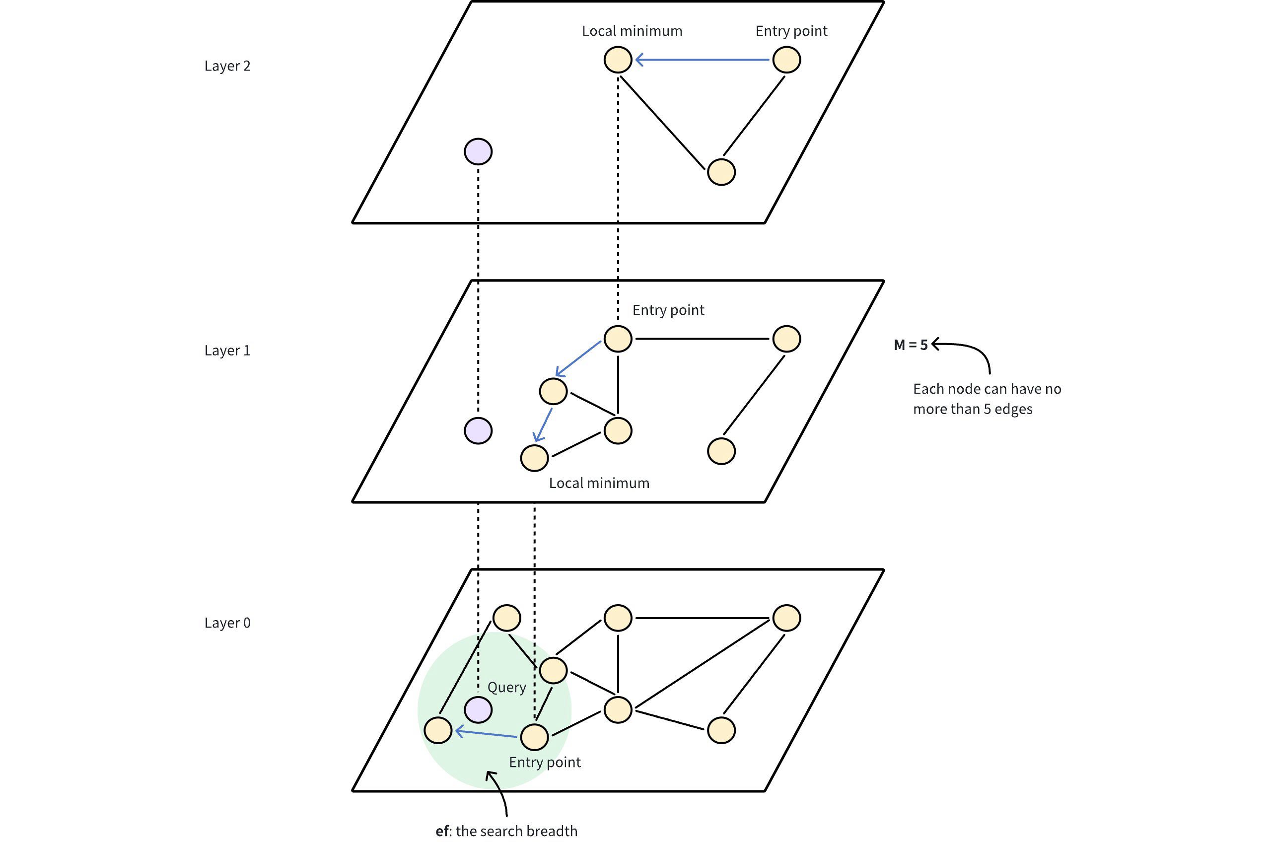
A simple way to conceptualize this is with nested collections, as shown in the Python example in the "Building HNSW from Scratch" article.

This nested dictionary-of-dictionaries model (vec2neighbors[vector_id][layer_num] = [neighbor_ids]) is perfect for understanding the logical relationships. However, for a high-performance C implementation, this approach is not ideal. It involves multiple levels of indirection and separate memory allocations, which can lead to poor data locality and cache performance. Your background in systems programming will tell you we can do better by designing a more compact and cache-friendly memory layout.

From Concept to C: A Cache-Friendly Design

To achieve high performance, we want to store as much of a node's essential data together in a contiguous block of memory as possible. A common and powerful technique in C for this kind of problem is to use a combination of structs and a flexible array member.

Let's look at a professional-grade implementation from Redis. The author of "Understanding Redis HNSW" breaks down the C structs used, which provide an excellent blueprint for our design. We'll separate the concerns into two structs:

1. hnswNodeLayer: Manages the connections for a single node on a single layer.
2. hnswNode: The main struct for a node, which will contain an array of hnswNodeLayer structs.

First, let's examine the hnswNodeLayer.

As you just read, the hnswNodeLayer is a compact structure that holds everything needed to manage a node's neighborhood on one level:

• struct hnswNode **links: A pointer to a dynamically allocated array of pointers. These pointers will point to the neighboring hnswNode structs.
• uint32_t num_links: The current number of neighbors in the links array.
• uint32_t max_links: The allocated capacity of the links array.

This max_links value is determined by the M parameter we've discussed. As a reminder, HNSW uses a larger number of connections on the base layer (Layer 0) to improve search accuracy. The Faiss video you watched previously confirms this common heuristic.

The Flexible Array Member Technique

Now, how do we combine this hnswNodeLayer with the main hnswNode? A node with a maximum layer l needs l+1 of these hnswNodeLayer structs (one for each layer from 0 to l). The number l is determined randomly at insertion time, so we can't just declare a fixed-size array in our hnswNode struct.

This is where the flexible array member comes in. It's a feature of C (since C99) that allows the last member of a struct to be an array of unspecified size. We can then allocate a single block of memory large enough for the struct and the desired number of elements for that array.

Let's return to the Redis HNSW article to see this in action.

This is the heart of our design. Let's break down the C code structure and the allocation process:

1. The Structs:
   We define our two primary structs. Note that hnswNodeLayer contains a pointer to hnswNode, so we need a forward declaration.

   // Forward-declare hnswNode so hnswNodeLayer can use a pointer to it.
   struct hnswNode;
   
   // Represents the connections for a node on a single layer.
   typedef struct {
       struct hnswNode **links;   // Dynamic array of pointers to neighbor nodes
       uint32_t num_links;        // Current number of neighbors
       uint32_t max_links;        // Allocated size of the links array (M or 2*M)
   } hnswNodeLayer;
   
   // Represents a single vector (a node) in the HNSW graph.
   typedef struct hnswNode {
       uint64_t id;               // Unique identifier for this node
       void *vector;              // Pointer to the actual vector data
       uint32_t level;            // The maximum layer this node exists on (our 'l')
       
       // ... other metadata for search, like 'visited_epoch' in the Redis example
       
       // Flexible array member: must be the last member of the struct.
       // This array will be sized at allocation time.
       hnswNodeLayer layers[];
   } hnswNode;
   

2. The Allocation:
   When we create a new node that has been assigned a maximum layer l, we perform a single memory allocation:
   newNode = malloc(sizeof(hnswNode) + sizeof(hnswNodeLayer) * (l + 1));

   This one malloc call reserves a contiguous block of memory that holds:

   • The fixed-size part of the hnswNode struct (id, vector pointer, level).
   • ...followed immediately by l + 1 instances of the hnswNodeLayer struct.

   We can then access the layers for this node using standard array syntax: newNode->layers[0], newNode->layers[1], ..., newNode->layers[l].

3. Initializing Connections:
   After this initial allocation, we must loop through each layer and allocate the links array for each one.

   // After allocating 'newNode' with max layer 'l'
   for (uint32_t i = 0; i <= l; i++) {
       uint32_t max_links_for_layer = (i == 0) ? M * 2 : M;
       newNode->layers[i].max_links = max_links_for_layer;
       newNode->layers[i].num_links = 0;
       
       // Now allocate the array of neighbor pointers for this layer
       newNode->layers[i].links = malloc(sizeof(struct hnswNode*) * max_links_for_layer);
   }
   

This design provides a superb balance of flexibility and performance. By co-locating the node's main data with its layer-specific connection metadata, we maximize the chances that accessing newNode->layers[i] will result in a cache hit if newNode was recently accessed. This is a crucial optimization for a search algorithm that will frequently traverse these structures.

Conclusion

In this lesson, we have translated the abstract requirement of storing a multi-layered graph into a concrete and performant C data structure design. You have seen how to move from a simple conceptual model to a sophisticated implementation that leverages low-level memory management for efficiency.

Key Takeaways:

• Logical Structure: A node must store a list of its neighbors for each layer it belongs to.
• C Implementation: This is best achieved with two structs: hnswNode for the main vector data and hnswNodeLayer for the connections on a single layer.
• Flexible Array Member: Using layers[] as the last member of hnswNode allows us to create a variably-sized object in a single, contiguous memory block.
• Contiguous Allocation: Allocating the hnswNode and its hnswNodeLayer array together (sizeof(hnswNode) + sizeof(hnswNodeLayer) * (l + 1)) significantly improves data locality and cache performance.
• Connection Limits: The max_links field in hnswNodeLayer is set based on the M parameter, typically with 2*M for layer 0 and M for higher layers.

We now have the "scaffolding" for our graph defined in memory. The next step is to build algorithms that operate on these structures. In the upcoming lesson, we will implement the SEARCH-LAYER algorithm, which is responsible for finding the nearest neighbors to a query vector within a single layer of the graph, making direct use of the layers[i].links arrays we designed today.