Optimized Cosine Similarity: SIMD Dot Product & L2 Norm

The Cosine Similarity Formula

Let's begin with the definition of Cosine Similarity. For two non-zero vectors $\mathbf{A}$ and $\mathbf{B}$, it is the cosine of the angle $\theta$ between them. Mathematically, it's defined as their dot product divided by the product of their magnitudes (their L2 norms):

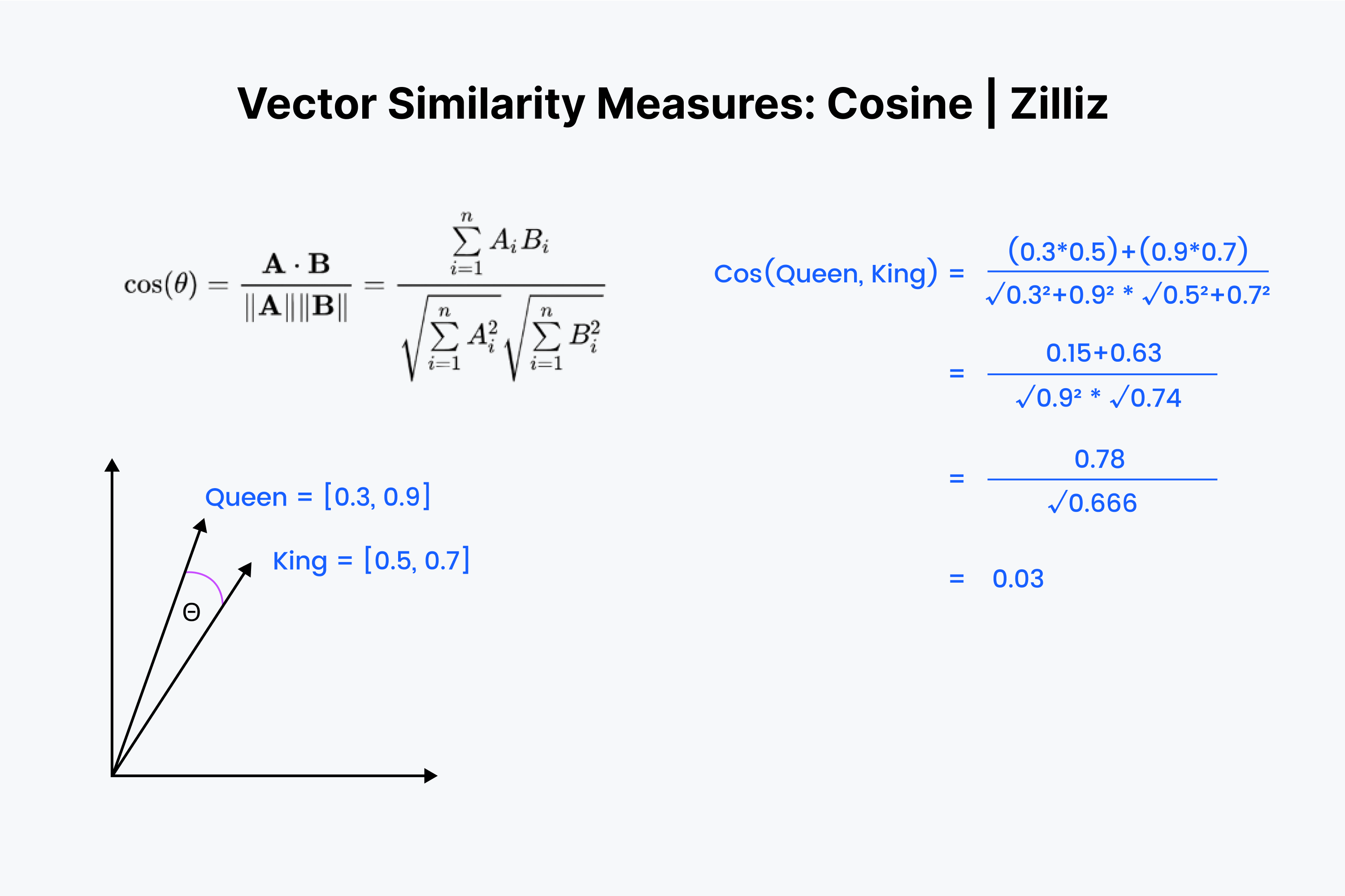
As you can see, the formula requires three distinct sums:

1. The dot product of $\mathbf{A}$ and $\mathbf{B}$ ($\sum A_i{B}_i$).
2. The sum of squares of $\mathbf{A}$'s elements ($\sum A_i^2$), which is the squared L2 norm of $\mathbf{A}$.
3. The sum of squares of $\mathbf{B}$'s elements ($\sum B_i^2$), the squared L2 norm of $\mathbf{B}$.

A straightforward way to implement this would be to call your existing dot_product and l2_norm_squared functions three times. While simple and modular, this "three-pass" approach is inefficient. It would require reading the vector data from memory three separate times, which can quickly become a bottleneck, especially for large vectors that don't fit in the CPU cache.

For high-performance systems, a much better strategy is the single-pass approach.

The Superiority of the Single-Pass Method

The core principle of the single-pass method is to calculate all three required sums simultaneously within a single loop. By loading chunks of vectors $\mathbf{A}$ and $\mathbf{B}$ just once, we can perform all the necessary multiplications and additions while the data is hot in the CPU registers. This drastically reduces the pressure on memory bandwidth and improves cache utilization.

The following blog post from SereneDB explains this exact trade-off.

This single-pass strategy is the standard for high-performance vector libraries and is exactly what we will implement.

Implementing the Single-Pass Cosine Similarity

To implement the single-pass method, we will integrate the logic from our previous two lessons into a single function. Instead of one set of accumulators for the dot product, we will now maintain three sets: one for the dot product ($A\cdot B$), one for the squared norm of A ($A\cdot A$), and one for the squared norm of B ($B\cdot B$).

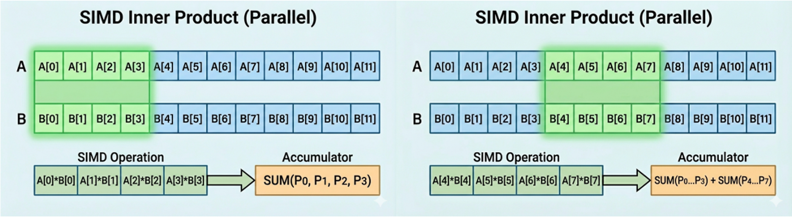
The following resource provides a C implementation that perfectly illustrates this technique.

The structure of your function will be:

1. Initialization: Create three __m256 registers, acc_ab, acc_a2, and acc_b2, and initialize them to zero using _mm256_setzero_ps(). If you were to apply the loop unrolling from our previous lessons, you would initialize 4 registers for each sum, for a total of 12 accumulator registers.

2. Main Loop: Iterate through the vectors, processing 8 floats (one __m256 register) at a time.

   • Load data: const __m256 a_chunk = _mm256_loadu_ps(a_ptr); and const __m256 b_chunk = _mm256_loadu_ps(b_ptr);.
   • Update accumulators using FMA:

     acc_ab = _mm256_fmadd_ps(a_chunk, b_chunk, acc_ab);
     acc_a2 = _mm256_fmadd_ps(a_chunk, a_chunk, acc_a2);
     acc_b2 = _mm256_fmadd_ps(b_chunk, b_chunk, acc_b2);
     

3. Horizontal Reduction: After the loop, you will have three __m256 registers containing partial sums. You need to perform the same horizontal sum procedure you learned for the dot product on each of these three registers to get three final scalar float values: sum_ab, sum_a2, and sum_b2.

4. Final Calculation: Compute the final result: sum_ab / (sqrtf(sum_a2) * sqrtf(sum_b2)). Remember to handle the edge case where a norm is zero to prevent division by zero.

Optimization: Reciprocal Square Root

The final division and square root operations can themselves be a performance bottleneck. Standard sqrtf() can be slow. A classic low-level optimization is to replace division by a square root with multiplication by its reciprocal.

Modern CPUs provide a dedicated instruction to compute the reciprocal of a square root, $1/\sqrt{x}$, which is much faster than a full square root followed by a division. In AVX, this is _mm_rsqrt_ps. This instruction is an approximation, so for better accuracy, it's standard practice to follow it with one or two rounds of Newton-Raphson refinement.

The "Understanding SIMD" article you just reviewed provides an excellent example of this.

Implementing this refinement shows a deep understanding of low-level optimization that is highly valued in performance engineering roles.

Conclusion

You have now assembled a complete, high-performance plan for calculating Cosine Similarity using SIMD. By moving from a naive three-pass approach to an efficient single-pass method, you've learned a critical pattern for optimizing data-intensive computations.

Key Takeaways:

• An efficient Cosine Similarity implementation calculates the dot product and both squared L2 norms within a single pass over the data.
• This is achieved by maintaining three sets of SIMD accumulator registers inside the main processing loop and updating them with FMA instructions.
• This approach minimizes memory bandwidth usage and maximizes cache efficiency.
• The final calculation can be further optimized by using the fast but approximate reciprocal square root instruction (_mm_rsqrt_ps), refined with a Newton-Raphson iteration for accuracy.

In our next lesson, we will put this all to the test. You will benchmark the performance of your naive and SIMD-accelerated distance functions to quantify the impressive speed gains you've achieved.