Entropy Changes in Ideal Gas Processes

Hello! Welcome back to our journey through thermodynamics.

In our last session, we got our hands dirty with the property tables and learned how to calculate the entropy change for pure substances like water. That was a huge practical step. We saw that for substances that change phase, the tables are our best friends.

But what about gases like air, nitrogen, or helium? In many real-world applications, from car engines to jet engines, these gases operate far from their condensation points. We can treat them as ideal gases. While we could use tables for them, it's often much faster and more insightful to use equations.

Today, we're going to derive and master the equations for calculating the entropy change of an ideal gas. This will give us a powerful new set of tools. By the end of our discussion, you'll be able to calculate how the entropy of a gas changes when you compress it, heat it, or expand it, and you'll understand why those changes happen.

From the General to the Specific: Finding the Master Equations

Remember how we said that entropy is a property, just like temperature or pressure? This means that its change depends only on the initial and final states, not the path taken. This is a crucial idea.

Even though entropy change itself is defined for a reversible process ( $d S = δ Q_{r e v} / T$ ), we can find general relationships between properties that are valid for any process. Let's find these master keys, often called the Tds relations or Gibbs Equations. This will feel a bit mathematical, but stick with me. The intuition we gain will be well worth it.

The First Tds Relation

Let's start with the First Law of Thermodynamics for a closed system undergoing a process:
$δ Q - δ W = d U$
This just says that the net energy crossing the boundary (heat in, work out) equals the change in the system's internal energy.
Now, let's imagine a reversible process. For this special case, we know two things:
- The heat transfer is $δ Q_{r e v} = T d S$ .
- The boundary work is $δ W_{r e v} = P d V$ .
Let's substitute these into the First Law:
$T d S - P d V = d U$
Rearranging this gives us our first master equation:
$T d S = d U + P d V$

Now for the magic trick. Look at this equation. It only contains properties: T, S, U, P, V. Since the relationship between properties doesn't depend on the path, this equation is true for any process that connects two equilibrium states, not just reversible ones. We used the idea of a reversible process to derive it, but the result is a general truth.

The Second Tds Relation

We can find another useful relation by using enthalpy, $H = U + P V$ .

Let's take the differential of the enthalpy definition:
$d H = d U + d (P V) = d U + P d V + V d P$
Notice that the term $d U + P d V$ is sitting right there. From our first Tds relation, we know that's equal to $T d S$ . Let's substitute it in:
$d H = T d S + V d P$
Rearranging gives us our second master equation:
$T d S = d H - V d P$

Just like the first one, this equation relates only properties, so it's universally valid for any process.

Okay, let's pause. We now have two powerful, general equations that connect entropy change to changes in other properties:

$T d S = d U + P d V$
$T d S = d H - V d P$

These are the starting point. Now, we'll apply them specifically to ideal gases.

Deriving the Entropy Change Equations for an Ideal Gas

This is where our knowledge of ideal gases from previous lessons comes into play. For an ideal gas, we know:

Change in internal energy: $d U = m C_{v} d T$
Change in enthalpy: $d H = m C_{p} d T$
The ideal gas law: $P V = m R T$

Let's plug these into our Tds relations.

Derivation 1: Starting with Internal Energy

Start with the first Tds relation: $T d S = d U + P d V$ .
Divide everything by T: $d S = \frac{d U}{T} + \frac{P}{T} d V$ .
Now, substitute the ideal gas facts:
- Replace dU with $m C_{v} d T$ .
- From the ideal gas law, $P / T = m R / V$ .
Our equation becomes:
$d S = m C_{v} \frac{d T}{T} + m R \frac{d V}{V}$
To find the total entropy change from state 1 to state 2, we integrate. Since you're comfortable with calculus, you'll see we're just summing up all the tiny dS changes.
$\int_{S_{1}}^{S_{2}} d S = \int_{T_{1}}^{T_{2}} m C_{v} \frac{d T}{T} + \int_{V_{1}}^{V_{2}} m R \frac{d V}{V}$
$Δ S = m (\int_{T_{1}}^{T_{2}} C_{v} (T) \frac{d T}{T} + R ln \frac{V _{2}}{V _{1}})$
Here, I've written $C_{v} (T)$ to remind us that specific heat can change with temperature.

Derivation 2: Starting with Enthalpy

Let's do the same thing with our second Tds relation for practice.

Start with $T d S = d H - V d P$ .
Divide by T: $d S = \frac{d H}{T} - \frac{V}{T} d P$ .
Substitute the ideal gas facts:
- Replace dH with $m C_{p} d T$ .
- From the ideal gas law, $V / T = m R / P$ .
Our equation becomes:
$d S = m C_{p} \frac{d T}{T} - m R \frac{d P}{P}$
Integrating from state 1 to state 2 gives us our second main equation for entropy change:
$Δ S = m (\int_{T_{1}}^{T_{2}} C_{p} (T) \frac{d T}{T} - R ln \frac{P _{2}}{P _{1}})$

Great! We now have two different (but equivalent) equations to calculate the entropy change of an ideal gas. One uses volume change, and the other uses pressure change.

The "Constant Specific Heats" Assumption

For many engineering problems, especially when the temperature change isn't huge, we can make a simplifying assumption: we can treat the specific heats, $C_{v}$ and $C_{p}$ , as constants. This makes the math much easier.

When $C_{v}$ and $C_{p}$ are constant, we can pull them out of the integral. The integral $\int_{1}^{2} \frac{d T}{T}$ simply becomes $ln (T_{2} / T_{1})$ .

This simplifies our two big equations into their most common forms. For the specific entropy change, $Δ s = Δ S / m$ :

Equation 1 (in terms of T and v):
$Δ s = C_{v} ln (\frac{T _{2}}{T _{1}}) + R ln (\frac{v _{2}}{v _{1}})$

Equation 2 (in terms of T and P):
$Δ s = C_{p} ln (\frac{T _{2}}{T _{1}}) - R ln (\frac{P _{2}}{P _{1}})$

These are your workhorse equations for ideal gas entropy problems. You choose which one to use based on whether you know the volumes or the pressures.

Let's explore what this means intuitively. The resource below provides a great summary of the final equations and an excellent "deep dive" on what entropy change means from a microscopic perspective.

Spontaneous Change: Entropy and Gibbs Energy

Let's read a short section from a Pearson physical chemistry resource. It will confirm the final equations we've just derived and also offer a beautiful microscopic explanation for why entropy increases when a gas expands.

Please read two parts of this document. First, read the section 'Changes in State for an Ideal Gas' (pages 592-593). Focus on the final derived equations, particularly equation (13.8), which is the same as our second equation. Then, read the 'ARE YOU WONDERING?' box on page 594. This gives a fantastic intuitive link between volume and entropy using the idea of microstates.

The microscopic view in that reading is so powerful, isn't it? When a gas expands into a larger volume, each molecule has more possible places it can be. The number of possible arrangements (microstates) skyrockets, and since entropy is a measure of these possibilities ( $S = k_{B} ln W$ ), the entropy increases. Our macroscopic formula $Δ s = R ln (v_{2} / v_{1})$ for an isothermal expansion is the direct mathematical consequence of this simple idea.

Putting It All Together: Special Cases

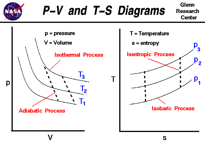
Let's see how these equations beautifully explain the entropy changes in the special processes we've already studied.

P-V and T-S Diagrams for Thermodynamic Processes — This image shows a P-V diagram (left) and a T-S diagram (right). The P-V diagram plots pressure vs. volume, showing curves for constant temperature (isotherms) and adiabatic processes. The T-S diagram plots temperature vs. specific entropy, showing lines for constant entropy (isentropic) and constant pressure (isobaric) processes. We'll use these to visualize our processes.

Isothermal Process (Constant Temperature, $T_{2} = T_{1}$ )
In our equations, the term $ln (T_{2} / T_{1})$ becomes $ln (1) = 0$ . So they simplify to:
- $Δ s = R ln (v_{2} / v_{1})$
- $Δ s = - R ln (P_{2} / P_{1})$
  This makes perfect sense. If you expand a gas isothermally ( $v_{2} > v_{1}$ ), its entropy increases. If you compress it ( $v_{2} < v_{1}$ ), its entropy decreases.
Isochoric Process (Constant Volume, $v_{2} = v_{1}$ )
Using Equation 1, the term $ln (v_{2} / v_{1})$ becomes $ln (1) = 0$ . The change is simply:
- $Δ s = C_{v} ln (T_{2} / T_{1})$
  If you heat the gas at constant volume, its entropy goes up. Cool it, and its entropy goes down.
Isobaric Process (Constant Pressure, $P_{2} = P_{1}$ )
Using Equation 2, the term $ln (P_{2} / P_{1})$ becomes $ln (1) = 0$ . The change is:
- $Δ s = C_{p} ln (T_{2} / T_{1})$
  Again, heating the gas at constant pressure increases its entropy.
Isentropic Process (Constant Entropy, $Δ s = 0$ )
This is the most interesting one. By definition, the entropy change is zero. Let's see what our equations tell us. Let's set Equation 2 to zero:
$0 = C_{p} ln (\frac{T _{2}}{T _{1}}) - R ln (\frac{P _{2}}{P _{1}})$
$C_{p} ln (\frac{T _{2}}{T _{1}}) = R ln (\frac{P _{2}}{P _{1}})$
Using logarithm rules ( $a ln x = ln x^{a}$ ):
$ln ((\frac{T _{2}}{T _{1}})^{C_{p}}) = ln ((\frac{P _{2}}{P _{1}})^{R})$
This means the terms inside the logs must be equal:
$(\frac{T _{2}}{T _{1}})^{C_{p}} = (\frac{P _{2}}{P _{1}})^{R}$
If we rearrange this using the ideal gas relations $R = C_{p} - C_{v}$ and $k = C_{p} / C_{v}$ , we can derive the famous isentropic relation we learned before:
$\frac{T _{2}}{T _{1}} = (\frac{P _{2}}{P _{1}})^{(k - 1) / k}$
This is fantastic! It shows that the isentropic relations are not just random formulas; they are the direct consequence of the entropy change being zero for an ideal gas.

Worked Problems

Let's solidify this with some practice. For air, we'll use these properties (you should memorize these for air):

Gas constant: $R = 0.287 kJ/kg\cdotK$
Constant pressure specific heat: $C_{p} = 1.005 kJ/kg\cdotK$
Constant volume specific heat: $C_{v} = 0.718 kJ/kg\cdotK$
Specific heat ratio: $k = 1.4$

Worked Problem 1: Compression in a Cylinder

Problem: 0.5 kg of air in a piston-cylinder is compressed from an initial state of 100 kPa and 25°C (298 K) to a final state of 600 kPa and 150°C (423 K). Calculate the total entropy change of the air.

Solution:
We are given the initial and final pressures and temperatures. This is a perfect setup to use our second entropy change equation.

Identify the Formula: We will use the equation involving T and P.
$Δ s = C_{p} ln (\frac{T _{2}}{T _{1}}) - R ln (\frac{P _{2}}{P _{1}})$
Plug in the Values: Remember to use absolute temperatures (Kelvin).
- $C_{p} = 1.005 kJ/kg\cdotK$
- $R = 0.287 kJ/kg\cdotK$
- $T_{1} = 298 K$ , $T_{2} = 423 K$
- $P_{1} = 100 kPa$ , $P_{2} = 600 kPa$
$Δ s = 1.005 ln (\frac{423}{298}) - 0.287 ln (\frac{600}{100})$
Calculate:
- $ln (423/298) = ln (1.4195) \approx 0.3503$
- $ln (600/100) = ln (6) \approx 1.7918$
$Δ s = (1.005 \times 0.3503) - (0.287 \times 1.7918)$
$Δ s = 0.3520 - 0.5143$
$Δ s = - 0.1623 kJ/kg\cdotK$
Find Total Entropy Change ( $Δ S$ ):
$Δ S = m \times Δ s = 0.5 kg \times (- 0.1623 kJ/kg\cdotK) = - 0.0812 kJ/K$

Intuitive Check: The entropy decreased. Does this make sense? The temperature increased (which tends to increase entropy), but the pressure increased significantly (which tends to decrease entropy by "squeezing" the molecules into a smaller effective space). In this case, the effect of the pressure increase was dominant, leading to a net decrease in the air's entropy.

Worked Problem 2: Heating in a Rigid Tank

Problem: A rigid tank contains air at 150 kPa and 20°C (293 K). The tank is heated until the pressure reaches 450 kPa. Find the change in specific entropy of the air.

Solution:
"Rigid tank" means the volume is constant ( $v_{1} = v_{2}$ ). This clues us in. We can use the simplified constant-volume formula, or the general one. Let's use the general one (Equation 1) and see that it simplifies.

Identify the Formula:
$Δ s = C_{v} ln (\frac{T _{2}}{T _{1}}) + R ln (\frac{v _{2}}{v _{1}})$
Since $v_{2} = v_{1}$ , the term $ln (v_{2} / v_{1}) = ln (1) = 0$ . So, it simplifies to:
$Δ s = C_{v} ln (\frac{T _{2}}{T _{1}})$
Find the Final Temperature ( $T_{2}$ ): We don't have $T_{2}$ , but we can find it. For a constant volume process with an ideal gas, the combined gas law tells us:
$\frac{P _{1} V _{1}}{T _{1}} = \frac{P _{2} V _{2}}{T _{2}} ⟹ \frac{P _{1}}{T _{1}} = \frac{P _{2}}{T _{2}}$
$T_{2} = T_{1} \times \frac{P _{2}}{P _{1}} = 293 K \times \frac{450 kPa}{150 kPa} = 293 \times 3 = 879 K$
Plug in the Values:
$Δ s = 0.718 ln (\frac{879}{293}) = 0.718 ln (3)$
$Δ s = 0.718 \times 1.0986 = 0.7888 kJ/kg\cdotK$

Intuitive Check: The entropy increased significantly. This makes sense, as the gas was heated to a very high temperature in a fixed volume, increasing its internal energy and molecular chaos.

Test your understanding!

Conceptual Question 1:
You take two identical samples of air. You heat the first sample at constant pressure by 50°C. You heat the second sample at constant volume by 50°C. Which sample experiences a larger increase in specific entropy? Why?

Show answer

The sample heated at constant pressure will have a larger entropy increase.
Here's why:

Formula Reason: The entropy change for constant pressure is $Δ s = C_{p} ln (T_{2} / T_{1})$ , and for constant volume it's $Δ s = C_{v} ln (T_{2} / T_{1})$ . Since $C_{p}$ is always greater than $C_{v}$ for an ideal gas (because some energy has to go into expansion work), the $Δ s$ for the constant pressure case will be larger.
Intuitive Reason: In the constant pressure case, the gas not only gets hotter, it also expands. This expansion gives the molecules more volume to roam in, which is an additional source of entropy increase on top of the heating. The constant volume case only has the entropy increase from heating.

A Note on Accuracy: Variable Specific Heats

Our assumption of constant specific heats is very convenient, but for processes with very large temperature changes, it can lead to some error. Realistically, $C_{p}$ and $C_{v}$ for gases do increase slightly with temperature.

How do we handle this? Engineers have pre-calculated the integral $\int C_{p} (T) / T d T$ and put the results in tables. This value is called the standard entropy, $s^{\circ} (T)$ . It's a property that depends only on temperature.

Using this, our second entropy equation becomes:
$Δ s = s_{2}^{\circ} - s_{1}^{\circ} - R ln \frac{P _{2}}{P _{1}}$
To solve a problem this way, you would:

Look up $s_{1}^{\circ}$ in the ideal gas table at temperature $T_{1}$ .
Look up $s_{2}^{\circ}$ at temperature $T_{2}$ .
Plug them into the formula.

This is the most accurate method for ideal gases. For our course, we will mostly stick to the constant specific heat assumption as it builds great intuition, but it's good to know this more precise method exists.

Key Takeaways

Fantastic work today. We've built a complete toolkit for calculating entropy change in ideal gases, all the way from first principles.

We started with the general Tds relations, $T d S = d U + P d V$ and $T d S = d H - V d P$ , which are true for any substance undergoing any process.
By applying ideal gas assumptions, we derived two key equations for calculating the change in specific entropy, $Δ s$ .
For the common case of constant specific heats, these equations are:
- $Δ s = C_{v} ln (T_{2} / T_{1}) + R ln (v_{2} / v_{1})$
- $Δ s = C_{p} ln (T_{2} / T_{1}) - R ln (P_{2} / P_{1})$
We saw how these equations simplify for isothermal, isochoric, and isobaric processes, and how they give rise to the isentropic relations when $Δ s = 0$ .

Preview of the Next Lesson

We've now learned how to calculate $Δ s$ for both pure substances (using tables) and ideal gases (using equations). But a picture is worth a thousand words. In our next lesson, we will introduce and master the Temperature-Entropy (T-s) diagram. This graphical tool will allow us to visualize thermodynamic processes and cycles in a whole new way, making concepts like isentropic efficiency and cycle analysis much more intuitive.

Recommended resources