Compressor and Pump Isentropic Efficiency

Hello again! It's great to see you back.

In our last lesson, we developed a powerful tool: isentropic efficiency. We saw how it allows us to give a performance score to a turbine by comparing the actual work it produces to the maximum possible work a "perfect" isentropic turbine could deliver. The formula, you'll remember, was:

$η_{T} = \frac{Actual Work Out}{Ideal Work Out} = \frac{W _{a}}{W _{s}} < 1$

Today, we're going to look at the other side of the coin. Instead of a device that produces work, like a turbine, we'll analyze devices that consume work: compressors and pumps. Think of the compressor in your air conditioner or refrigerator, or the water pump that supplies your home. Their job is to increase the pressure of a fluid, and that requires an energy input.

Our goal for this lesson is to define and calculate the isentropic efficiency of a compressor or pump. The core idea is the same—comparing real performance to an ideal benchmark—but we'll discover a crucial twist in how we define it.

The Twist: Efficiency for Work-Consuming Devices

Let's go back to our performance score analogy. For a turbine (a work producer), the ideal case gives you the most work. So, you compare what you actually got to that maximum possible value.

But for a compressor or pump, the goal is different. You want to achieve a certain pressure increase while putting in the least amount of work possible. The ideal, isentropic process represents this minimum required work. The real-world process, with all its friction and turbulence, will always require more work to get the same job done.

So, if we have:

Ideal (Isentropic) Work Input = $W_{s}$ (the minimum possible)
Actual Work Input = $W_{a}$ (what you really have to supply)

We know that $W_{a} > W_{s}$ . If we used the same formula as the turbine, $W_{a} / W_{s}$ , we'd get an efficiency greater than 100%, which doesn't make sense.

To keep our efficiency score as a value between 0 and 1 (or 0% and 100%), we have to flip the fraction. We compare the best-case scenario (minimum work) to the real-world scenario (actual work):

η_{C} = \frac{Isentropic (Ideal) Work Input}{Actual Work Input} = \frac{W _{s}}{W _{a}}

The subscript 'C' stands for compressor. The same logic applies to a pump, which is essentially just a compressor for liquids.

To see this explained concisely, let's watch a short segment from a familiar channel.

Turbines, Compressors, and Pumps - ISENTROPIC EFFICIENCY in 8 Minutes!

The 'Less Boring Lectures' video we saw last time also covers compressors. This first part clearly explains why the efficiency formula for a compressor is 'inverted' compared to a turbine.

Please watch from 0:34 to 1:05. Focus on the core logic: to get a number between 0 and 1, the smaller quantity (ideal work) must go in the numerator.

Visualizing Compressor Efficiency on an h-s Diagram

Let's see what this looks like on an enthalpy-entropy (h-s) diagram. A compressor takes a fluid at a low pressure ( $P_{1}$ ) and raises it to a high pressure ( $P_{2}$ ).

Isentropic Efficiency of Adiabatic Compressors and Pumps on an h-s Diagram — This h-s diagram illustrates the process for an adiabatic compressor. The fluid starts at state 1. The ideal, isentropic process is a vertical line up to the higher pressure line, ending at state 2s. This represents the minimum work input, $w_s = h_{2s} - h_1$. The real, irreversible process generates entropy, so the path moves up and to the right, ending at state 2a. This requires a larger work input, $w_a = h_{2a} - h_1$.

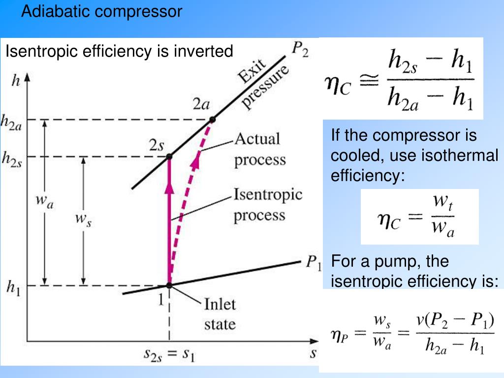
From the diagram, you can clearly see:

The isentropic work input ( $w_{s}$ ) corresponds to the vertical enthalpy rise, $h_{2 s} - h_{1}$ . This is the minimum possible energy required.
The actual work input ( $w_{a}$ ) corresponds to the larger enthalpy rise, $h_{2 a} - h_{1}$ .
The difference, $h_{2 a} - h_{2 s}$ , is the extra work you had to supply that got converted into heat by irreversibilities (friction, etc.), making the fluid hotter at the exit than it would have been ideally.

The Calculation Formula for Compressors

Now we can derive our main formula. We start with the First Law for a steady-flow device (our compressor), assuming it's adiabatic with negligible changes in kinetic and potential energy. The work input per unit mass ( $w$ ) is:

$w = h_{e x i t} - h_{in l e t}$

Applying this to our two cases:

Actual Work Input: $w_{a} = h_{2 a} - h_{1}$
Isentropic Work Input: $w_{s} = h_{2 s} - h_{1}$

Substituting these into our inverted efficiency definition, we get the isentropic efficiency for a compressor:

η_{C} = \frac{w _{s}}{w _{a}} = \frac{h _{2 s} - h _{1}}{h _{2 a} - h _{1}}

Let's watch two more clips that walk through this visualization and derivation in detail. The diagram used is a T-s diagram, but the vertical axis represents temperature instead of enthalpy. For an ideal gas, they are directly proportional, so the shape and logic are identical.

Thermodynamics: Isentropic Efficiencies for Turbine, Compressor, Pump

This video by Raili Taylor provides a great step-by-step walkthrough. It shows the process on a T-s diagram and derives the final enthalpy formula.

Please watch from 15:56 to 18:17. The first part visualizes the ideal and actual processes. The second part puts it all together to arrive at the efficiency formula in terms of enthalpy.

The Special Case: Pumps and Incompressible Liquids

Pumps follow the exact same efficiency logic as compressors. However, for practical calculations, we often use a simplified approach. Why? Because the fluid is a liquid (like water), and liquids are nearly incompressible. This means their specific volume ( $v$ ) barely changes even when pressure increases dramatically.

Also, detailed property tables for compressed (or subcooled) liquids are not always as readily available as those for gases and steam.

This incompressibility gives us a fantastic shortcut to find the ideal work input ( $w_{s}$ ). For a reversible process, we know the work is the integral of $v d P$ . Since $v$ is constant for an incompressible fluid, the integral becomes very simple:

$w_{s} = \int_{1}^{2} v d P \approx v_{1} (P_{2} - P_{1})$

This gives us the ideal, isentropic work input for a pump. The actual work input, $w_{a}$ , is still best found from the actual enthalpy change, $w_{a} = h_{2 a} - h_{1}$ .

So, the isentropic efficiency for a pump ( $η_{P}$ ) is often written as:

η_{P} = \frac{w _{s}}{w _{a}} = \frac{v _{1} ( P _{2} - P _{1} )}{h _{2 a} - h _{1}}

This is an extremely useful formula in practice. The video we just saw explains this exact point.

Thermodynamics: Isentropic Efficiencies for Turbine, Compressor, Pump

Let's continue with the same video, as it explains this special treatment for pumps.

Please watch from 19:31 to 21:55. The key takeaway is how the assumption of an incompressible fluid simplifies the ideal work calculation to v \Delta P.

Worked Numerical Problems

Time to put these formulas into practice.

Problem 1: Compressing a Refrigerant

Problem Statement: Refrigerant-134a enters an adiabatic compressor as a saturated vapor at -20°C. It is compressed to a pressure of 1.0 MPa. If the isentropic efficiency of the compressor is 85%, determine the actual work input per unit mass (in kJ/kg) and the temperature of the refrigerant at the exit.

Step-by-Step Solution

We'll follow a similar process to our turbine problems, but using the compressor efficiency formula.

1. Fix State 1 (Inlet):

We are given that the fluid is R-134a, and the state is saturated vapor at $T_{1} = - 2 0^{\circ} C$ .
We go to the saturated R-134a tables (temperature table). At $- 2 0^{\circ} C$ , we are at the "saturated vapor" column (subscript 'g').
From the tables, we find:
- Pressure, $P_{1} = 132.82 kPa$
- Enthalpy, $h_{1} = h_{g} = 238.41 kJ/kg$
- Entropy, $s_{1} = s_{g} = 0.9456 kJ/kg\cdotK$

2. Find the Ideal Exit State (2s):

We know the exit pressure is $P_{2} = 1.0 MPa = 1000 kPa$ .
For the ideal isentropic process, $s_{2 s} = s_{1} = 0.9456 kJ/kg\cdotK$ .
Now we go to the superheated R-134a tables at $P_{2} = 1.0 MPa$ . We look for our entropy value, $s_{2 s}$ . We'll likely have to interpolate.
- At $T = 4 0^{\circ} C$ , $s = 0.9156$ kJ/kg·K and $h = 272.05$ kJ/kg.
- At $T = 5 0^{\circ} C$ , $s = 0.9479$ kJ/kg·K and $h = 282.74$ kJ/kg.
Our value $s_{2 s} = 0.9456$ is between these two points. Let's interpolate to find $h_{2 s}$ :
$\frac{h _{2 s} - 272.05}{282.74 - 272.05} = \frac{0.9456 - 0.9156}{0.9479 - 0.9156}$
$\frac{h _{2 s} - 272.05}{10.69} = \frac{0.0300}{0.0323} = 0.9288$
$h_{2 s} = 272.05 + 0.9288 \times 10.69 = 272.05 + 9.92 = 281.97 kJ/kg$
(We can also interpolate for $T_{2 s}$ , which would be around 49.3°C, but we need $h_{2 s}$ for the work calculation).

3. Calculate the Isentropic Work Input ( $w_{s}$ ):
$w_{s} = h_{2 s} - h_{1} = 281.97 - 238.41 = 43.56 kJ/kg$
This is the absolute minimum work required.

4. Calculate the Actual Work Input ( $w_{a}$ ):

We are given the efficiency, $η_{C} = 0.85$ .
Rearrange the efficiency formula to solve for $w_{a}$ : $η_{C} = w_{s} / w_{a} ⟹ w_{a} = w_{s} / η_{C}$
$w_{a} = \frac{43.56 kJ/kg}{0.85} = 51.25 kJ/kg$
The actual work required is 51.25 kJ/kg.

5. Find the Actual Exit State (2a):

We can find the actual exit enthalpy $h_{2 a}$ from the actual work:
$w_{a} = h_{2 a} - h_{1} ⟹ h_{2 a} = h_{1} + w_{a} = 238.41 + 51.25 = 289.66 kJ/kg$
Now, we go back to the superheated R-134a tables at $P_{2} = 1.0 MPa$ and find the temperature corresponding to this enthalpy ( $h_{2 a} = 289.66$ kJ/kg).
- At $T = 5 0^{\circ} C$ , $h = 282.74$ kJ/kg.
- At $T = 6 0^{\circ} C$ , $h = 293.38$ kJ/kg.
Our value is between these. Let's interpolate for the actual exit temperature, $T_{2 a}$ :
$\frac{T _{2 a} - 50}{60 - 50} = \frac{289.66 - 282.74}{293.38 - 282.74} = \frac{6.92}{10.64} = 0.650$
$T_{2 a} = 50 + 0.650 \times 10 = 56. 5^{\circ} C$
The actual exit temperature is 56.5°C. Notice this is significantly hotter than the ideal exit temperature would have been (~49.3°C).

Problem 2: Pumping Water

Problem Statement: Water enters a pump at 100 kPa as a saturated liquid. It is pumped to a pressure of 4 MPa. The mass flow rate is 0.5 kg/s. If the isentropic efficiency of the pump is 78%, what is the actual power required by the pump in kW?

Step-by-Step Solution

Here we'll use our special pump formula.

1. Fix State 1 (Inlet):

We are given water at $P_{1} = 100 kPa$ as a saturated liquid.
We go to the saturated water tables (pressure table). At 100 kPa, we look at the "saturated liquid" column (subscript 'f').
We need the specific volume $v_{1}$ and enthalpy $h_{1}$ .
- $v_{1} = v_{f} = 0.001043 m^{3} /kg$
- $h_{1} = h_{f} = 417.51 kJ/kg$

2. Calculate the Isentropic Work Input ( $w_{s}$ ):

We use our incompressible liquid formula: $w_{s} \approx v_{1} (P_{2} - P_{1})$ .
Crucially, ensure units are consistent! Pressure must be in kPa to match the kJ unit. $1 MPa = 1000 kPa$ . $1 kJ = 1 kPa \cdot m^{3}$ .
$P_{2} = 4 MPa = 4000 kPa$ .
$w_{s} = (0.001043 m^{3} /kg) (4000 kPa - 100 kPa)$
$w_{s} = (0.001043) (3900) = 4.068 kJ/kg$
This is the minimum work required to pump the water.

3. Calculate the Actual Work Input ( $w_{a}$ ):

We are given $η_{P} = 0.78$ .
$w_{a} = \frac{w _{s}}{η _{P}} = \frac{4.068 kJ/kg}{0.78} = 5.215 kJ/kg$

4. Calculate the Actual Power Required ( $W ˙_{a}$ ):

Power is work per unit time. We multiply the work per unit mass by the mass flow rate.
$W ˙_{a} = m ˙ \times w_{a} = (0.5 kg/s) (5.215 kJ/kg) = 2.608 kJ/s = 2.61 kW$
The actual power required by the pump is 2.61 kW.

Test your understanding!

Using the results from Problem 2, what is the temperature of the water leaving the pump? (Hint: First find $h_{2 a}$ , then use the compressed liquid tables, or make an approximation).

Show answer

First, let's find the actual enthalpy of the water leaving the pump, $h_{2 a}$ .
$w_{a} = h_{2 a} - h_{1} ⟹ h_{2 a} = h_{1} + w_{a} = 417.51 + 5.215 = 422.725 kJ/kg$
Now we need to find the temperature for water at $P_{2} = 4 MPa$ and $h_{2 a} = 422.725 kJ/kg$ . This is a compressed liquid state.
From the saturated tables, the saturation temperature at 100 kPa (our inlet) is $T_{s a t} = 99.6 1^{\circ} C$ .
Looking at the compressed liquid tables for water at 5 MPa (close enough to 4 MPa for an estimate), the enthalpy of saturated liquid at 100°C is ~419 kJ/kg. Our enthalpy is slightly higher. This indicates the temperature will be slightly higher than the inlet temperature of 99.61°C.
Specifically, for compressed liquids, temperature doesn't change much with pressure, but it does change with enthalpy. The increase in enthalpy due to the work input causes a very slight temperature rise. Without detailed tables, we can definitively say the exit temperature will be slightly above 99.61°C. Using software, the answer is approximately 99.7°C. The key insight is that pumping a liquid adds a lot of pressure but only slightly increases its temperature.

Conceptual Questions

1. You have two identical compressors operating between the same inlet state and the same exit pressure. Compressor A is cooled (heat is removed during compression), while Compressor B is adiabatic (perfectly insulated). Which compressor would you expect to require less work input? Why?

Answer:
Compressor A (the cooled one) would require less work. Think back to the h-s or T-s diagram. The work input is the change in enthalpy. Cooling the gas during compression lowers its temperature and enthalpy at any given pressure. This has the effect of "pulling down" the process line on the diagram, reducing the overall vertical distance ( $h_{2} - h_{1}$ ) and thus reducing the work required. This is why large industrial compressors often have cooling jackets or intercoolers.

2. Why is the actual exit temperature of an adiabatic compressor always higher than the ideal isentropic exit temperature?

Answer:
The isentropic process is the "perfect" ideal, with no friction or other irreversibilities. In a real adiabatic compressor, those irreversibilities are unavoidable. The extra energy that must be supplied to overcome friction and turbulence doesn't just disappear; it is converted into internal energy within the fluid, causing its final enthalpy and temperature to be higher than the ideal case. It's "wasted" work that ends up as extra heat.

3. An engineer designs a pump and claims its isentropic efficiency is 95%. They then design a compressor and also claim its isentropic efficiency is 95%. Does this mean the two devices are equally "good" at their jobs?

Answer:
Yes. The isentropic efficiency is a standardized measure of performance relative to the ideal. A 95% efficient pump is achieving 95% of its ideal goal (which is to use the minimum work, so it's using $1/0.95 = 1.053$ times the ideal minimum work). A 95% efficient turbine is also achieving 95% of its ideal goal (producing 95% of the maximum possible work). Both are performing at an exceptionally high level, very close to their respective thermodynamic limits.

Key Takeaways for Today

Excellent work! We've now completed our understanding of isentropic efficiency for the core components of thermodynamic cycles.

Efficiency for Work-Consumers: For compressors and pumps, the goal is to minimize work input. Therefore, the efficiency definition is "flipped" to keep the value below 1:
$η_{C, P} = \frac{Ideal (Isentropic) Work}{Actual Work} = \frac{W _{s}}{W _{a}}$
Compressor Formula: In terms of properties, this is $η_{C} = (h_{2 s} - h_{1}) / (h_{2 a} - h_{1})$ .
Pump Formula: For pumps handling incompressible liquids, we use the practical formula $η_{P} = v_{1} (P_{2} - P_{1}) / (h_{2 a} - h_{1})$ .
Real vs. Ideal: In a real adiabatic compressor or pump, irreversibilities cause the actual work input and the final fluid temperature to be higher than in the ideal isentropic case.

Preview of the Next Lesson

So far, we've analyzed turbines, compressors, and pumps in isolation. But in the real world, these devices don't work alone. They are connected together to form cycles that continuously produce power or move heat.

In our next lesson, we will begin our study of Gas Power Cycles. We'll start with the foundational cycle for most car engines: the Otto cycle. We'll see how the processes we've learned—compression, heat addition, expansion, and heat rejection—can be combined to create a complete engine cycle. See you then

Recommended resources