The Definite Integral as a Limit of Riemann Sums

1. From an Infinite Number of Rectangles to Exact Area

In the previous lesson, we saw that as we increase $n$, the number of rectangles, our approximation of the area under the curve gets better. The over- or under-estimated regions become smaller.

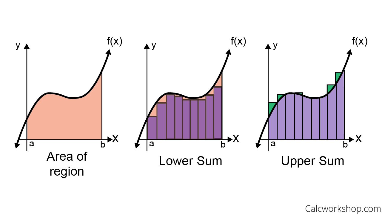
This naturally leads to a question: what happens if we let the number of rectangles, $n$, go to infinity? Intuitively, the width of each rectangle, $\Delta x$, would become infinitesimally small, and the sum of their areas would perfectly match the area under the curve.

This process of taking a limit is the cornerstone of defining the exact area. The following video provides a concise introduction to this leap from approximation to a formal definition.

2. The Formal Definition of the Definite Integral

As the video showed, we define the exact area under the curve of a continuous function $f(x)$ from $x=a$ to $x=b$ as the limit of a Riemann sum.

This limit is given a special name and notation: the definite integral.

To see the formal definition laid out, please read the following short section.

Let's break down this crucial definition. If a function $f(x)$ is continuous on the interval $[a,b]$, we divide the interval into $n$ subintervals of equal width $\Delta x=(b-a)/n$. We then choose a sample point $x_i^{\ast }$ in each subinterval $[x_{i-1},x_i]$. This sample point could be the left endpoint, right endpoint, midpoint, or any other point within the subinterval.

The definite integral of $f$ from $a$ to $b$ is:

This equation is packed with meaning:

• ${\int }_a^b\dots dx$ is the integral sign. The numbers $a$ and $b$ are called the limits of integration, representing the start and end of the interval.
• The elongated 'S' of the integral sign, $\int$, evolved from the summation sign, $\sum$, signifying an infinite sum.
• $f(x)$ is the integrand, the function whose curve we are finding the area under.
• $dx$ represents an infinitesimally small width of a rectangle, evolving from $\Delta x$ as $n\to \infty$. It also indicates that $x$ is the variable of integration.

The entire expression ${\int }_a^{b}f(x)dx$ is read as "the integral of f of x from a to b". When the function is non-negative, this value is the exact area under the curve. If the function dips below the x-axis, the integral calculates the signed area, where areas below the axis are counted as negative.

3. A More Rigorous Perspective

For most practical purposes, defining the integral as the limit as $n\to \infty$ with equal subintervals is sufficient. However, the truly rigorous mathematical definition is a bit more general and powerful. It ensures that the approximation improves no matter how we partition the interval, as long as all partitions become fine enough.

This more general approach considers that subintervals don't have to be of equal width. Instead of taking the limit as $n\to \infty$, we take the limit as the width of the widest sub-interval approaches zero. This width is called the "size" or "norm" of the partition.

The following video explains this more general and robust definition. While it goes into more detail, it solidifies the concept that for a continuous function, the limit is the same no matter which Riemann sum you use (left, right, midpoint, irregular).

The key theorem presented in the video is profound: for a continuous function on a closed interval, the definite integral exists, and its value is unique. It doesn't matter if you use left-hand sums, right-hand sums, or some other method; as you refine the partitions, they all converge to the same value.

4. Rewriting a Limit as a Definite Integral

A key skill is to recognise the limit of a Riemann sum and write it in the more compact definite integral notation. This involves identifying the function $f(x)$, the interval $[a,b]$, and the differential $dx$.

Let's break down the example in the image:
${\lim }_{n\to \infty }{\sum }_{i=1}^n\left[{\left(2+\frac{5i}{n}\right)}^2+2\right]\frac{5}{n}$

1. Identify $\Delta x$: The term multiplying the whole expression is $\Delta x=\frac{5}{n}$. Since $\Delta x=\frac{b-a}{n}$, we know that the length of our interval is $b-a=5$.

2. Identify $x_i$: The general form for the right endpoint is $x_i=a+i\Delta x$. In our expression, we see the term $2+\frac{5i}{n}$. Comparing this to $a+i\frac{5}{n}$, we can deduce that the starting point is $a=2$.

3. Determine the Interval $[a,b]$: Since $a=2$ and $b-a=5$, we find that $b=2+5=7$. So, our interval of integration is $[2,7]$.

4. Identify the Function $f(x)$: The function is what's being done to the $x_i$ term. Here, the term $(2+\frac{5i}{n})$ is being squared and then has 2 added to it. So, $f(x_i)=(x_i{)}^2+2$. This means our function is $f(x)=x^2+2$.

Putting it all together, the limit of the sum is equivalent to the definite integral:
${\int }_2^7(x^2+2)dx$

Conclusion

In this lesson, we made the crucial transition from approximating area to defining it exactly.

Key Takeaways:

• The definite integral, ${\int }_a^{b}f(x)dx$, represents the exact signed area between the curve of $f(x)$ and the x-axis over the interval $[a,b]$.
• It is formally defined as the limit of a Riemann sum:
  ${\int }_a^{b}f(x)dx={\lim }_{n\to \infty }{\sum }_{i=1}^{n}f(x_i^{\ast })\Delta x$
• For a continuous function, this limit has a unique value, regardless of how the subintervals are partitioned or which sample points ($x_i^{\ast }$) are chosen, as long as the widest subinterval shrinks to zero.

You may be thinking that calculating these limits looks incredibly difficult and tedious. You would be right! It is not the practical way to find the value of an integral.

In our next lesson, we will introduce a revolutionary idea: the Fundamental Theorem of Calculus. This theorem provides an astonishingly simple method for evaluating definite integrals, directly linking this "area problem" back to the antiderivatives we studied just a few lessons ago.