Estimating Area with Riemann Sums

1. The Area Problem

Imagine you have a function, say $y=f(x)$, and you want to find the exact area of the region under its graph, bounded by the x-axis and two vertical lines at $x=a$ and $x=b$.

If the function were a simple horizontal line (forming a rectangle) or a straight diagonal line (forming a trapezium/trapezoid), you could use basic geometry. But what if the top boundary is a curve?

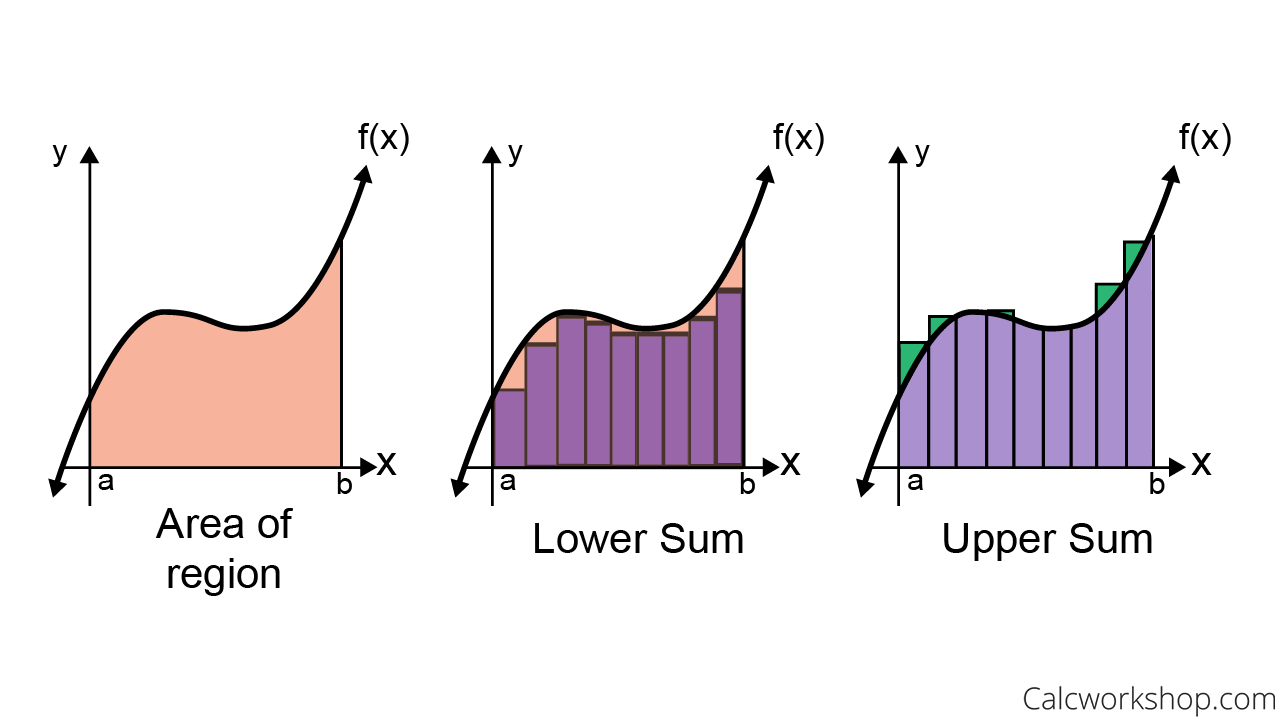
The fundamental idea, as shown in the image above, is to approximate this irregular area by filling it with a shape we do know how to measure: the rectangle. By summing the areas of several rectangles, we can get a good estimate of the total area. This sum is called a Riemann Sum, named after the 19th-century German mathematician Bernhard Riemann.

2. Building the Approximation

To create our rectangular approximation, we follow a systematic process:

1. Partition the Interval: We take the interval on the x-axis from $a$ to $b$ and divide it into $n$ smaller subintervals of equal width. The width of each of these subintervals is denoted by $\Delta x$.

   $$\Delta x=\frac{b-a}{n}$$

   Here, $n$ is the number of rectangles we choose to use.

2. Determine the Heights: For each subinterval, we draw a rectangle whose base is $\Delta x$. The crucial question is: how tall should each rectangle be? The height is determined by the value of the function $f(x)$ at a specific point within that subinterval. There are three common conventions for choosing this point.

3. Left, Right, and Midpoint Riemann Sums

The three most common methods for determining the height of the rectangles are the Left-hand Rule, the Right-hand Rule, and the Midpoint Rule.

Let's define each one. We'll label the endpoints of our subintervals as $x_0,x_1,x_2,\dots ,x_n$, where $x_0=a$ and $x_n=b$.

• Left Riemann Sum ($L_n$): The height of each rectangle is determined by the function's value at the left endpoint of the subinterval.
  The total area is:
  $L_n=f(x_0)\Delta x+f(x_1)\Delta x+\dots +f(x_{n-1})\Delta x={\sum }_{i=0}^{n-1}f(x_i)\Delta x$

• Right Riemann Sum ($R_n$): The height of each rectangle is determined by the function's value at the right endpoint of the subinterval.
  The total area is:
  $R_n=f(x_1)\Delta x+f(x_2)\Delta x+\dots +f(x_n)\Delta x={\sum }_{i=1}^{n}f(x_i)\Delta x$

• Midpoint Riemann Sum ($M_n$): The height of each rectangle is determined by the function's value at the midpoint of the subinterval. If we call the midpoint of the $i$-th interval ${\bar{x}}_i$, the area is:
  $M_n=f({\bar{x}}_1)\Delta x+f({\bar{x}}_2)\Delta x+\dots +f({\bar{x}}_n)\Delta x={\sum }_{i=1}^{n}f({\bar{x}}_i)\Delta x$
  where ${\bar{x}}_i=\frac{x_{i-1}+x_i}{2}$.

4. A Worked Example

Seeing these rules in action makes them much clearer. The following video provides an excellent, step-by-step demonstration of how to calculate the Left, Right, and Midpoint Riemann sums for a specific function.

After watching the video, let's try a problem.

5. The Formal Definition of a Riemann Sum

So far, we have only considered partitions with equal subinterval widths and specific choices for the height (left, right, or midpoint). The formal definition of a Riemann Sum is more general.

To get a formal handle on this, the following resource from The Open University provides a clear, concise definition.

In its most general form, a Riemann sum doesn't require the subintervals to be of equal width. Furthermore, the point $c_i$ chosen within each subinterval $[x_{i-1},x_i]$ to determine the rectangle's height can be any point in that subinterval, not just an endpoint or midpoint.

A general Riemann Sum is therefore:

where $\Delta x_i$ is the width of the $i$-th subinterval and $c_i$ is any sample point within it. For our purposes in this course, we will almost always use subintervals of equal width ($\Delta x$), as it simplifies the calculations significantly.

6. Improving the Approximation

It seems logical that using more, narrower rectangles would give a better approximation of the area. As we increase $n$, the number of rectangles, our sum gets closer to the true area under the curve. The error in our approximation—the small regions that are either over- or under-counted—gets smaller and smaller.

This leads to a profound idea: what if we could use an infinite number of rectangles? If we take the limit of the Riemann sum as the number of rectangles $n$ approaches infinity (and thus the width of each rectangle $\Delta x$ approaches zero), we should get the exact area.

Conclusion

In this lesson, we have built the machinery to approximate the area under a curve.

Key Takeaways:

• The area under a curve can be approximated by summing the areas of multiple rectangles, a method known as a Riemann sum.
• The interval $[a,b]$ is divided into $n$ subintervals, each forming the base of a rectangle with width $\Delta x=(b-a)/n$.
• The height of each rectangle can be determined using different rules, most commonly the Left-hand Rule, Right-hand Rule, or Midpoint Rule.
• Increasing the number of rectangles ($n$) generally leads to a more accurate approximation of the area.

This concept of approximating area is the crucial stepping stone to our next topic. We will see how the limit of a Riemann sum as $n\to \infty$ gives us the exact area and leads to the formal definition of the definite integral.