Solving Logarithmic Equations

1. The Most Important Rule: Check Your Answers!

Before we even solve our first equation, we need to address a crucial feature of logarithms. The argument of a logarithm must always be positive.

Think about the definition: if $y={\log }_b(x)$, it means $b^y=x$. Since the base $b$ is always a positive number (and not 1), raising it to any real power $y$ will always result in a positive number $x$.

This means that any solution we find for $x$ must not cause the argument of any logarithm in the original equation to be zero or negative. A "solution" that does so is called an extraneous root and must be discarded.

For this reason, when solving logarithmic equations, it is not just recommended to check your answers—it is essential.

2. The Core Strategies for Solving

There are two primary strategies for solving logarithmic equations, both of which stem from the properties of logarithms. The goal is almost always to manipulate the equation into one of these two forms:

1. Form 1: log_b (A) = C (A logarithm equals a number)
   • Strategy: Convert the equation into its exponential form, A = b^C, and then solve for the variable. This uses the fundamental inverse relationship between logs and exponentials.

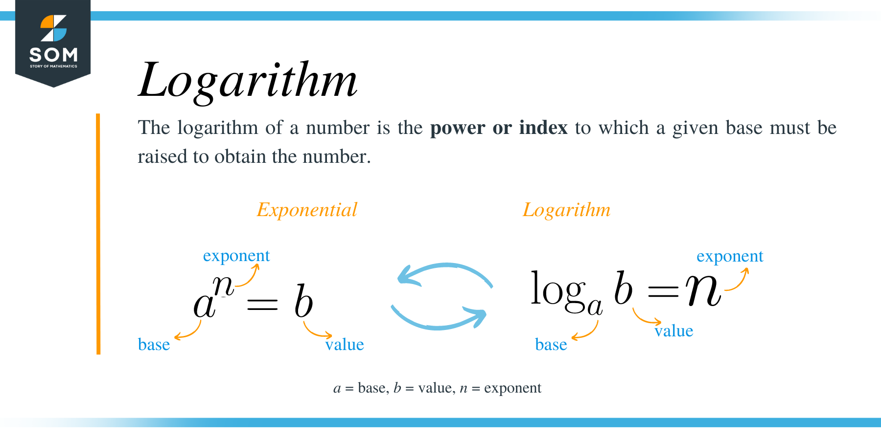
*This image illustrates the direct conversion between logarithmic and exponential forms, which is the basis for our first strategy.*

2. Form 2: log_b (A) = log_b (B) (A logarithm equals another logarithm with the same base)
* Strategy: Use the one-to-one property of logarithms. If the logs are equal and the bases are the same, then the arguments must be equal. Set A = B and solve.

Let's see these strategies in action.

3. Strategy 1: Logarithm = Number

This is the most direct type of logarithmic equation.

Example: Solve log_5 (2x - 3) = 2.

1. Identify the form: This is log_b(A) = C, where b=5, A = 2x - 3, and C = 2.
2. Convert to exponential form: 2x - 3 = 5^2.
3. Solve for x: $$\begin{gathered} 2x-3=25 \\ 2x=28 \\ x=14 \end{gathered}$$
4. Check the solution: Substitute x=14 back into the original argument: 2(14) - 3 = 28 - 3 = 25. Since 25 is positive, the solution is valid.

4. Strategy 2: Logarithm = Logarithm

When an equation has a single logarithm on each side with the same base, the solution is often straightforward.

Example: Solve log(x^2 - 1) = log(8). (Remember, log with no base written is the common logarithm, base 10).

1. Identify the form: This is log_b(A) = log_b(B).
2. Set arguments equal: x^2 - 1 = 8.
3. Solve for x: $$\begin{gathered} x^2=9 \\ x=3\text{or}x=-3 \end{gathered}$$
4. Check both solutions:
   • For x = 3: The argument is 3^2 - 1 = 8, which is positive. Valid.
   • For x = -3: The argument is (-3)^2 - 1 = 9 - 1 = 8, which is positive. Also valid.

In this case, we have two valid solutions.

5. Combining the Rules: Condensing Logarithms

Most problems won't start in one of the simple forms. You'll first need to use the laws of logarithms (product, quotient, and power rules) to condense the expression into a single logarithm on one or both sides.

Example 1: Using the Product Rule

Solve log_6(x + 2) + log_6(x + 3) = 1.

1. Condense: The sum of two logs is the log of their product.
   ${\log }_6((x+2)(x+3))=1$
2. Identify the form: The equation is now log_b(A) = C.
3. Convert to exponential form: (x + 2)(x + 3) = 6^1.
4. Solve for x: This results in a quadratic equation. $$\begin{gathered} x^2+5x+6=6 \\ {x}^2+5x=0 \\ x(x+5)=0 \end{gathered}$$ The potential solutions are x = 0 and x = -5.
5. Check both solutions:
   • For x = 0: The original arguments are 0+2 = 2 (positive) and 0+3 = 3 (positive). Valid.
   • For x = -5: The original arguments are -5+2 = -3 (negative) and -5+3 = -2 (negative). Since this makes the arguments negative, x = -5 is an extraneous root.

The only solution is x = 0.

Example 2: Using the Quotient and Power Rules

Solve log_2(x+2) - log_2(x-5) = 3.

1. Condense: The difference of two logs is the log of their quotient.
   ${\log }_2\left(\frac{x+2}{x-5}\right)=3$
2. Identify the form: This is log_b(A) = C.
3. Convert to exponential form: \frac{x+2}{x-5} = 2^3.
4. Solve for x: $$\begin{gathered} \frac{x+2}{x-5}=8 \\ x+2=8(x-5) \\ x+2=8x-40 \\ 42=7x \\ x=6 \end{gathered}$$
5. Check the solution: For x = 6, the original arguments are 6+2=8 (positive) and 6-5=1 (positive). Valid.

The solution is x = 6.

Conclusion

In this lesson, we developed a systematic approach to solving logarithmic equations. By mastering the core strategies and being diligent with checking your work, you can confidently solve a wide range of problems.

Key Takeaways:

• The Golden Rule: The argument of any logarithm must be positive. Always check your final answers in the original equation to discard any extraneous roots.
• Condense First: Use the laws of logarithms (product, quotient, power rules) to combine multiple logs into a single logarithm on each side of the equation.
• Two Core Strategies:
  1. If the equation is in the form log_b(A) = C, convert it to exponential form A = b^C and solve.
  2. If the equation is in the form log_b(A) = log_b(B), set the arguments equal, A = B, and solve.

Preview of the Next Lesson:

The concept of ensuring a logarithm's argument is positive is a specific instance of a much broader and more fundamental idea in mathematics: the domain of a function. In our next lesson, we will begin the "Understanding Functions" module. We will learn how to formally identify a function and determine its domain and range from an equation or a graph, generalising the ideas we've used today.