Exponential Functions: Graphs & Properties

1. What is an Exponential Function?

An exponential function is a function of the form:
$f(x)=a^x$
where:

• a is a constant called the base.
• x is the variable, which is in the index (or exponent).

This structure is the reverse of what we've seen in polynomials. Before we explore their behaviour, we need to establish some important rules about the base a.

To summarise the key constraints on the base a:

• a must be positive (a > 0). If the base were negative, the function would oscillate between positive and negative values (e.g., $(-2{)}^1=-2$, $(-2{)}^2=4$), resulting in a disconnected graph that is not useful for modelling continuous growth or decay.
• a cannot be 1. If a=1, the function becomes $f(x)=1^x=1$, which is just a constant horizontal line.

Therefore, for exponential functions, we only consider bases where a > 0 and a ≠ 1. This leaves us with two main categories to investigate: a > 1 and 0 < a < 1.

Evaluating these functions relies heavily on the rules of indices (powers) you learned back in Module 2. As a quick refresher:

• $a^0=1$ (Any non-zero base to the power of 0 is 1)
• $a^{-n}=\frac{1}{a^n}$ (A negative index indicates a reciprocal)
• $a^{1/n}=\sqrt[n]{a}$ (A fractional index indicates a root)

2. Graphing and Analysing Exponential Functions

The best way to understand the properties of exponential functions is to see them visually. We'll build the graphs by plotting points calculated from their equations.

Case 1: Exponential Growth (a > 1)

As you saw in the video, when the base a is greater than 1, the function value increases as x increases. This is called exponential growth.

Let's look at the graph of $y=2^x$.

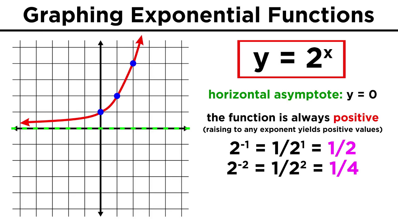
Based on the video and this graph, let's identify the key properties for functions like $y=2^x$ and $y=3^x$, where a > 1:

• Domain: You can put any real number x into the function, so the domain is $(-\infty ,\infty )$.
• Range: The output y is always positive. The graph never touches or crosses the x-axis. The range is $(0,\infty )$.
• Y-intercept: The graph always crosses the y-axis at the point (0, 1), because $a^0=1$ for any base a.
• Horizontal Asymptote: The graph gets closer and closer to the x-axis ($y=0$) as x becomes more negative ($x\to -\infty$). The line $y=0$ is a horizontal asymptote.
• Behaviour (Behavior): The function is always increasing. As x increases, y increases.
• Key Point: The graph always passes through the point (1, a), because $a^1=a$. For $y=2^x$, this is the point (1, 2). For $y=3^x$, it's (1, 3).

When comparing $y=2^x$ and $y=3^x$, notice that for $x>0$, the graph of $y=3^x$ is steeper. For $x<0$, the graph of $y=3^x$ is closer to the x-axis.

Case 2: Exponential Decay (0 < a < 1)

What happens when the base is a fraction between 0 and 1?

This is called exponential decay. When 0 < a < 1, the function value decreases as x increases.

A crucial insight here is the connection to negative indices. Remember that $(1/2{)}^x$ can be written as $(2^{-1}{)}^x$, which simplifies to $2^{-x}$. This means the graph of $y=(1/2{)}^x$ is a reflection of the graph of $y=2^x$ in the y-axis.

The properties are very similar to the growth case:

• Domain: $(-\infty ,\infty )$
• Range: $(0,\infty )$
• Y-intercept: Still at (0, 1).
• Horizontal Asymptote: The x-axis ($y=0$), but this time the graph approaches it as x becomes more positive ($x\to \infty$).
• Behaviour (Behavior): The function is always decreasing. As x increases, y decreases.
• Key Point: The graph still passes through (1, a). For $y=(1/2{)}^x$, this is the point (1, 1/2).

This image provides a great summary of the general characteristics for all exponential functions of the form $f(x)=a^x$.

3. The Natural Exponential Function: e^x

In your scientific and IT work, you will frequently encounter one special base: the number e. This is an irrational number, like $\pi$, and it's also known as Euler's number.

Its value is approximately:
$e\approx \mathrm{2.71828...}$

The function $f(x)=e^x$ is called the natural exponential function. It's arguably the most important exponential function because it arises naturally in many areas of calculus, finance, and science.

Since $e\approx 2.718$, the base is greater than 1. This means the function $f(x)=e^x$ has all the properties of an exponential growth function:

• It is an increasing function.
• It passes through the key points (0, 1) and (1, e).
• It has a horizontal asymptote at $y=0$.
• Its graph lies between the graphs of $y=2^x$ and $y=3^x$.

You can calculate values of $e^x$ on most scientific calculators, usually using a button labelled e^x.

Conclusion

In this lesson, we have introduced the family of exponential functions, $f(x)=a^x$. We established that their behaviour is determined by the value of the base a.

Key Takeaways:

• An exponential function has the form $f(x)=a^x$, where a is a positive constant not equal to 1.
• If a > 1, the function represents exponential growth. It is always increasing.
• If 0 < a < 1, the function represents exponential decay. It is always decreasing. The graph of $y=(1/a{)}^x$ is a reflection of $y=a^x$ in the y-axis.
• All exponential functions $f(x)=a^x$ share these common properties:
  • Domain: All real numbers.
  • Range: All positive real numbers ($y>0$).
  • They pass through the point (0, 1).
  • They have a horizontal asymptote at the x-axis ($y=0$).
• The function $f(x)=e^x$, where $e\approx 2.718$, is the natural exponential function and is a case of exponential growth.

Preview of the Next Lesson:
Now that we have a solid understanding of exponential functions, a natural question arises: if we know the output y, can we find the input x that produced it? This involves finding the inverse of the exponential function. In our next lesson, we will define the logarithm as the inverse of an exponential function and learn how to move between exponential and logarithmic forms.