Vectorized Operations in NumPy

1. The Need for Speed: What is Vectorization?

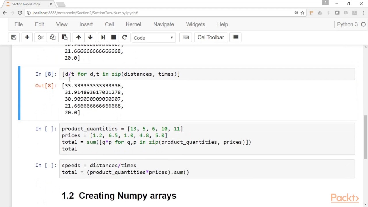
Given your background in computer science, you're familiar with the performance differences between interpreted and compiled languages. A standard Python for loop, while flexible, can be slow when processing large amounts of numerical data. Each iteration requires the interpreter to perform type checks and other overhead, creating a significant bottleneck.

Vectorization is the technique of applying an operation to an entire array at once, rather than element by element. In NumPy, these operations are executed by highly optimized, pre-compiled C code. This pushes the iterative work into a much faster, lower-level layer, leading to dramatic speed improvements.

The following video provides an excellent conceptual overview of vectorization and demonstrates its real-world impact.

As the video highlights, the benefits of vectorization come from:

1. Executing operations in parallel: Using multiple CPU cores to process chunks of the array simultaneously.
2. Using homogeneous data types: NumPy arrays contain elements of a single type (e.g., all int64 or all float64), which eliminates Python's type-checking overhead and allows for C-level optimizations.
3. Ensuring memory locality: NumPy arrays are stored in a contiguous block of memory, which allows for faster access compared to Python lists, whose elements can be scattered throughout memory.

The result is not just faster code, but also code that is cleaner and easier to read.

2. NumPy's Universal Functions (Ufuncs)

Now, let's put this into practice. The primary way to perform vectorized operations in NumPy is through its Universal Functions, or ufuncs. These are functions that operate on NumPy arrays in an element-by-element fashion.

The following resource provides a detailed look at how these functions work.

As you've read, we can categorize these operations into two main types:

Unary Operations

These functions take a single array as input and produce a new array as output.

Example:

import numpy as np




# Create an array of temperatures in Celsius
celsius = np.array([0, 10, 20, 30, 100])




# Unary operations like square root
# np.sqrt(celsius) # This would work, but let's do a more practical example next.

Binary Operations

These functions take two arrays (or an array and a scalar) as input and produce a new array. When operating on two arrays, the operation is performed on corresponding elements.

Example:
Let's convert our Celsius temperatures to Fahrenheit using the formula $F=C\times \frac{9}{5}+32$.

# Binary operations: array and scalar
fahrenheit = celsius * 1.8 + 32

print(fahrenheit)



# Expected output: array([ 32.,  50.,  68.,  86., 212.])

Notice how we didn't need to write a for loop. The multiplication (*) and addition (+) were applied to every element in the celsius array. This is vectorization in action.

3. Broadcasting: A Powerful Feature

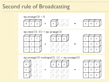
So far, our binary operations have involved either two arrays of the exact same shape or an array and a single number (a scalar). But what if you want to perform an operation between arrays of different but compatible shapes? This is where broadcasting comes in.

Broadcasting describes the rules for how NumPy treats arrays with different shapes during arithmetic operations. In short, NumPy "broadcasts" the smaller array across the larger array so that they have compatible shapes.

This short video provides a clear, visual explanation of the rules.

The core rules of broadcasting are:

1. If the arrays do not have the same number of dimensions, the shape of the one with fewer dimensions is padded with ones on its leading (left) side.
2. If the shape of the two arrays does not match in any dimension, the array with shape equal to 1 in that dimension is stretched to match the other shape.
3. If in any dimension the sizes disagree and neither is equal to 1, an error is raised.

Your Turn: Practice Vectorized Operations

Let's apply these concepts with a quick exercise.

Imagine you have sales data for a set of products. You have the number of units sold per day in one array and the price per unit in another.

import numpy as np




# Units sold each day for 5 days
units_sold = np.array([50, 65, 42, 88, 56])




# Price per unit
price = 19.99




# 1. Calculate the total revenue for each day.
#    The result should be a new NumPy array.
daily_revenue = units_sold * price
print("Daily Revenue:", daily_revenue)





# Now, let's use broadcasting. Suppose you have prices for three different products
# in a 2D array, representing sales over two days.
sales_data = np.array([
    [10, 15, 8],  # Day 1: sales for product A, B, C
    [12, 18, 11]  # Day 2: sales for product A, B, C
])




# You are given a 1D array of taxes per product.
taxes = np.array([0.50, 0.75, 0.40]) # Tax for product A, B, C




# 2. Add the tax to the sales data for each respective product.
#    NumPy should broadcast the 'taxes' array across the rows of 'sales_data'.
total_cost_with_tax = sales_data + taxes
print("\nSales Data with Tax:\n", total_cost_with_tax)

Run this code and analyze the output. Make sure you understand how the taxes array was broadcast across the sales_data array. The shape of sales_data is (2, 3) and the shape of taxes is (3,). Broadcasting aligns them and performs the addition.

Conclusion

In this lesson, you've grasped the essential concept of vectorization, which underpins all high-performance numerical computing in Python.

Key Takeaways:

• Vectorization is the process of applying operations to entire arrays at once, which is significantly faster than using Python loops.
• This speed comes from using pre-compiled C code, leveraging homogeneous data types, and ensuring data is stored in contiguous memory blocks.
• NumPy's Universal Functions (ufuncs) provide an intuitive way to perform element-wise mathematical operations (e.g., +, *, np.sqrt).
• Broadcasting provides flexible rules for applying operations to arrays of different but compatible shapes, avoiding the need for manual array reshaping.

These concepts are the bedrock upon which the Pandas library is built. As we move forward, you'll see that operations you perform on Pandas Series and DataFrames are, under the hood, fast vectorized NumPy operations.

In the next lesson, we will begin our journey with Pandas. You'll learn how to create, select, and manipulate data in Pandas Series and DataFrames using loc, iloc, and boolean indexing. This is where we start working with the labeled, tabular data structures that are central to data analysis in Python.