Missing Data Handling Techniques

1. Understanding and Identifying Missing Data

Before we fix the problem, it's crucial to understand why it happens and how to find it. Missing data isn't just a nuisance; it can tell a story. For instance, why might a user not report their income in a survey? The reason could influence how you decide to handle that missing value.

This article provides a great conceptual overview of missing data.

Now that you have the conceptual background, let's look at a map of the techniques we'll explore. This flowchart provides an excellent overview of the different paths you can take when confronted with missing values.

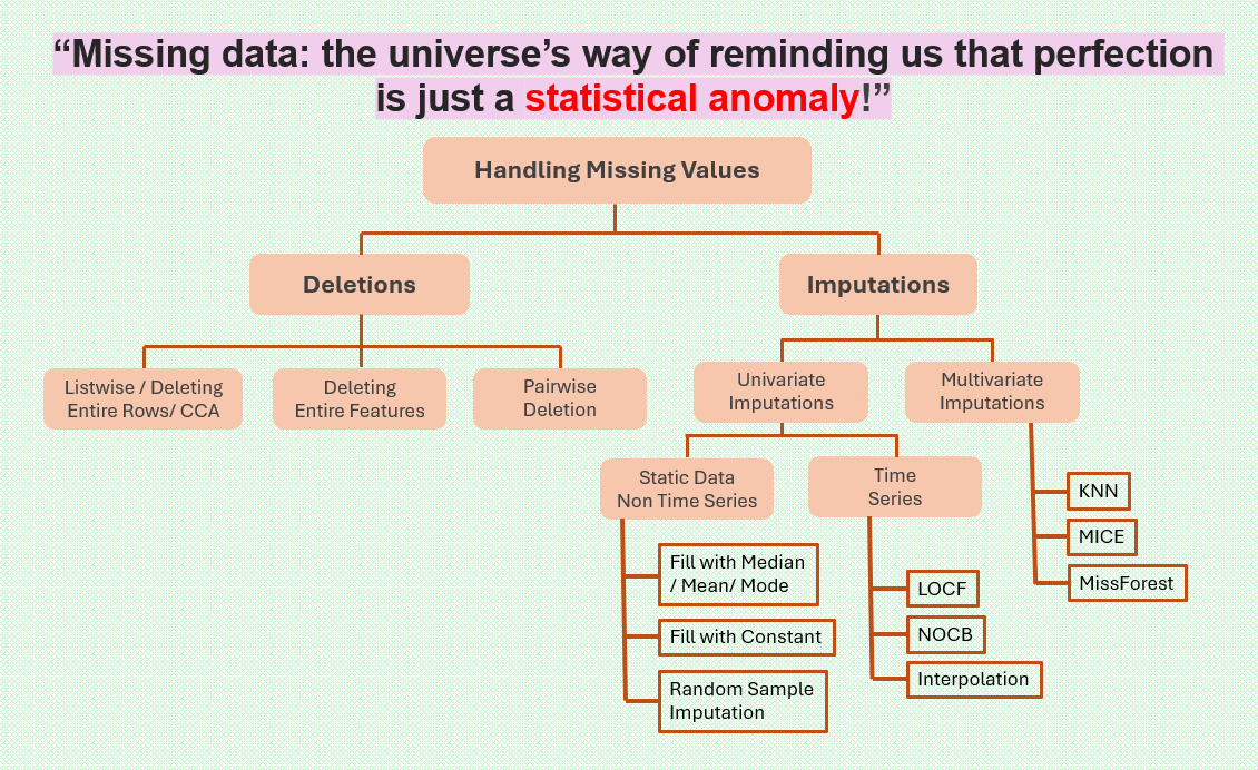
The first practical step is to identify where the missing values are in your DataFrame. Pandas makes this easy with the .isnull() method (an alias for .isna()), which returns a boolean DataFrame. We typically chain this with .sum() to get a count of missing values per column.

import pandas as pd
import numpy as np




# Sample DataFrame with various missing values
data = {
    'product': ['A', 'B', 'C', 'D', 'E'],
    'price': [100, 120, np.nan, 150, 110],
    'category': ['Elec', 'Elec', 'Home', np.nan, 'Home'],
    'sales_last_month': [50, np.nan, 20, 35, np.nan]
}
df = pd.DataFrame(data)

print("Original DataFrame:")
print(df)
print("\n" + "="*30 + "\n")




# Check for missing values
print("Boolean mask of missing values:")
print(df.isnull())
print("\n" + "="*30 + "\n")




# Get a count of missing values per column
print("Count of missing values per column:")
print(df.isnull().sum())

2. Deletion Strategies: The dropna() Method

The most straightforward approach is to simply remove rows or columns that contain missing data. This is known as listwise deletion when dropping rows.

• Pros: It's simple and fast. If the amount of missing data is very small, it might not significantly harm your dataset.
• Cons: You lose data. If the missing values are not randomly distributed, you could introduce bias into your analysis.

The dropna() method is your tool for this. The following video gives a fantastic, detailed walkthrough of its most important parameters.

3. Imputation Strategies: Filling in the Gaps

Instead of deleting data, we can often make an educated guess to fill in, or impute, the missing values. This preserves your sample size but requires careful thought. The video below covers the most common imputation functions in Pandas.

To complement the video, let's summarize the main imputation techniques.

a) Filling with a Constant, Mean, or Median

• Constant: Use df.fillna(0) or df.fillna('Unknown'). This is simple but can distort the column's statistical properties.
• Mean/Median: A more robust approach for numerical data is to fill with the column's mean or median. The median is often preferred as it's less sensitive to outliers.

Here is how you would apply it:

# Create a sample DataFrame
df_numeric = pd.DataFrame({'scores': [88, 92, np.nan, 75, 95, 85, np.nan]})




# Fill with the mean
mean_imputed = df_numeric['scores'].fillna(df_numeric['scores'].mean())
print("Mean Imputed:\n", mean_imputed)




# Fill with the median (more robust to outliers)
median_imputed = df_numeric['scores'].fillna(df_numeric['scores'].median())
print("\nMedian Imputed:\n", median_imputed)

b) Forward and Backward Fill (ffill, bfill)

As you saw in the codebasics video, these methods are excellent for ordered data (like time series), where you can assume a missing value is the same as the one immediately before or after it.

c) Interpolation

The interpolate() method is a step up from ffill/bfill for numerical, ordered data. It fills NaN values by treating them as points on a line between the known values. This often provides a more realistic estimate than simply carrying a previous value forward.

4. Case Study: Cleaning Real-World Survey Data

Now, let's apply these concepts to a realistic scenario. In the previous lesson, you learned to handle custom missing values like "not available" during import using na_values. What happens when your data contains strings that aren't technically missing, but prevent numerical analysis?

The following segment from Corey Schafer's video walks through a perfect example using Stack Overflow survey data to calculate the average years of coding experience.

This example is a powerful illustration of a typical data cleaning workflow: identify a problem, investigate its root cause, apply targeted cleaning steps, and then proceed with your analysis.

Conclusion

You now have a solid toolkit for one of the most common tasks in data science: handling missing data. There is no single "best" method; the right choice is always context-dependent.

Key Takeaways:

• Identify First: Always start by using .isnull().sum() to understand the extent of missing data in your dataset.
• Deletion (dropna): A quick and easy solution, but use with caution. It's best when the amount of missing data is small. The subset parameter gives you fine-grained control.
• Imputation (Filling): A powerful way to preserve data. Your main tools are:
  • fillna(): For constants, statistical measures (mean/median), or propagation (method='ffill'/'bfill').
  • interpolate(): For smarter filling of ordered numerical data.
• Context is King: The choice of strategy depends on the data type (numeric vs. categorical), the nature of the data (e.g., time series), and the potential reasons for the data being missing.

In our next lesson, we'll build directly on this. Now that you know how to load and clean your data, we'll learn how to perform summary statistics and initial data inspection using .info(), .describe(), and .value_counts(). This will allow us to quickly understand the main characteristics of our dataset before diving into more complex analysis and visualization.