Linear Regression Basics

1. The Core Idea: Fitting a Line to Data

At its heart, linear regression is about finding the best-fitting straight line through a set of data points. This "line of best fit" represents the relationship between your input features (e.g., the square footage of a house) and the target you want to predict (e.g., its price).

But how does the algorithm decide which line is "best"? It uses a method called Ordinary Least Squares (OLS). The concept is highly intuitive and is explained brilliantly in the following video from StatQuest.

To summarize the key ideas from the video:

• The goal of linear regression is to find the parameters—a slope and an intercept—for a line that minimizes the sum of the squared distances between each data point and the line.
• The equation for this line (in the simple case of one feature) is: $$\text{prediction}=(\text{coefficient}\times \text{feature})+\text{intercept}$$
• R-squared ($R^2$) measures the proportion of the variance in the dependent variable that is predictable from the independent variable(s). A score of 1.0 means the model perfectly explains the data's variance, while a score of 0.0 means it explains none.

2. Training a Linear Regression Model with Scikit-learn

Now, let's translate this theory into practice. We'll build a pipeline to predict house prices using the popular California Housing dataset, which is conveniently available in scikit-learn.

Since you are now proficient with pipelines, our workflow should look familiar: we'll scale our features and then pass them to the linear regression model.

Here is the code to get started. I've set up the data loading and train-test split. Your task is to define and train the pipeline.

import pandas as pd
import numpy as np
from sklearn.datasets import fetch_california_housing
from sklearn.model_selection import train_test_split
from sklearn.preprocessing import StandardScaler
from sklearn.linear_model import LinearRegression
from sklearn.pipeline import Pipeline
from sklearn.metrics import r2_score, mean_absolute_error, mean_squared_error




# 1. Load the dataset
housing = fetch_california_housing(as_frame=True)
X = housing.data
y = housing.target




# 2. Split the data
X_train, X_test, y_train, y_test = train_test_split(X, y, test_size=0.2, random_state=42)




# 3. Define the pipeline
# Create a pipeline with two steps:
# 'scaler': a StandardScaler to scale the features
# 'model': a LinearRegression model
lr_pipeline = Pipeline([
    ('scaler', StandardScaler()),
    ('model', LinearRegression())
])




# 4. Train the pipeline
lr_pipeline.fit(X_train, y_train)




# 5. Make predictions on the test set
y_pred = lr_pipeline.predict(X_test)

print("Pipeline training complete.")

By fitting this pipeline, you've trained your first linear regression model. The StandardScaler learned the mean and standard deviation from the training data, and the LinearRegression model found the optimal coefficients (slopes) and intercept to minimize the squared errors on that same scaled training data.

3. Interpreting the Model's Predictions

Training a model is only half the battle; interpreting its results is where you derive real-world insights. Let's break down how to understand what your model has learned.

A. Model Coefficients

The trained model stores the intercept and the coefficient for each feature. We can access them from the model step in our pipeline.

• Intercept: The baseline predicted value if all feature values were zero.
• Coefficients: The "weights" the model assigns to each feature.

# Access the fitted model from the pipeline
model = lr_pipeline.named_steps['model']




# Get the intercept
intercept = model.intercept_
print(f"Intercept: {intercept:.4f}")




# Get the coefficients and pair them with feature names
coefficients = pd.DataFrame({
    'feature': X.columns,
    'coefficient': model.coef_
}).sort_values(by='coefficient', ascending=False)

print("\nModel Coefficients:")
print(coefficients)

How to Interpret the Coefficients:

Since we used StandardScaler, the interpretation is as follows: "A one standard deviation increase in a feature results in a change in the predicted house price equal to that feature's coefficient (in hundreds of thousands of dollars), assuming all other features remain constant."

For example:

• A large positive coefficient (like for MedInc, median income) means that higher median income in a block group is strongly associated with a higher predicted house price.
• A large negative coefficient (like for AveOccup, average occupancy) suggests that more crowded households are associated with lower predicted house prices.

B. Model Performance Metrics

How good are our predictions? We can use several metrics to evaluate the model's performance on the unseen test data.

# Calculate R-squared: The proportion of variance explained by the model
r2 = r2_score(y_test, y_pred)




# Calculate Mean Absolute Error (MAE): The average absolute difference between predicted and actual values.
# It's easy to interpret as it's in the original units of the target.
mae = mean_absolute_error(y_test, y_pred)




# Calculate Root Mean Squared Error (RMSE): The square root of the average of squared differences.
# It's also in the original units but penalizes larger errors more heavily.
rmse = np.sqrt(mean_squared_error(y_test, y_pred))

print(f"\nR-squared (R2) on Test Set: {r2:.4f}")
print(f"Mean Absolute Error (MAE) on Test Set: {mae:.4f}")
print(f"Root Mean Squared Error (RMSE) on Test Set: {rmse:.4f}")

• An $R^2$ of around 0.59 means our model explains about 59% of the variability in California house prices. This is a decent, but not perfect, fit.
• An MAE of about 0.53 means that, on average, our model's predictions are off by about $53,000 (since the target is in units of $100,000).

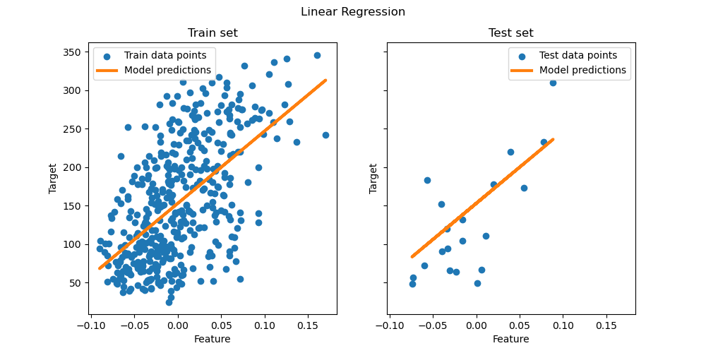
This visualizes what we've done. The model (orange line) captures the general trend in both the training and testing data.

C. Statistical Significance of Features (Advanced Interpretation)

Scikit-learn's LinearRegression is optimized for prediction. It doesn't provide statistical summaries, like p-values, which tell us if a feature's coefficient is statistically significant. For this, data scientists often turn to the statsmodels library.

The statsmodels library provides a detailed summary that is invaluable for interpretation.

Here's what a statsmodels OLS summary looks like:

Key things to look for in this summary are:

• R-squared: Confirms the model's overall fit.
• coef: The coefficient values, which should be very similar to what we got from scikit-learn.
• P>|t|: This is the p-value for each coefficient. The null hypothesis is that the coefficient is zero (i.e., the feature has no effect). A p-value less than 0.05 is a standard threshold to reject this hypothesis, suggesting the feature is a statistically significant predictor.

Using statsmodels allows you to report not just what the model predicts, but also how confident you can be in the contribution of each feature to that prediction.

Conclusion

In this lesson, you have moved from preprocessing theory to practical model building. You trained your first supervised learning model, a linear regression, and learned how to interpret it from multiple angles.

Key Takeaways:

• Linear regression models the relationship between features and a continuous target by fitting a line that minimizes the sum of squared errors (residuals).
• The trained model has an intercept (baseline value) and coefficients (weights) for each feature, which tell you the direction and magnitude of each feature's effect.
• Model performance is evaluated with metrics like $R^2$ (proportion of variance explained) and error metrics like MAE and RMSE (prediction error in the target's units).
• While scikit-learn is excellent for building predictive models, the statsmodels library is the tool of choice for in-depth statistical inference, providing p-values to assess the significance of each feature.

In our next lesson, we will shift from regression to classification. You'll learn how to predict categorical outcomes (e.g., yes/no, spam/not spam) using Logistic Regression, an algorithm that cleverly adapts the linear model for this new task.