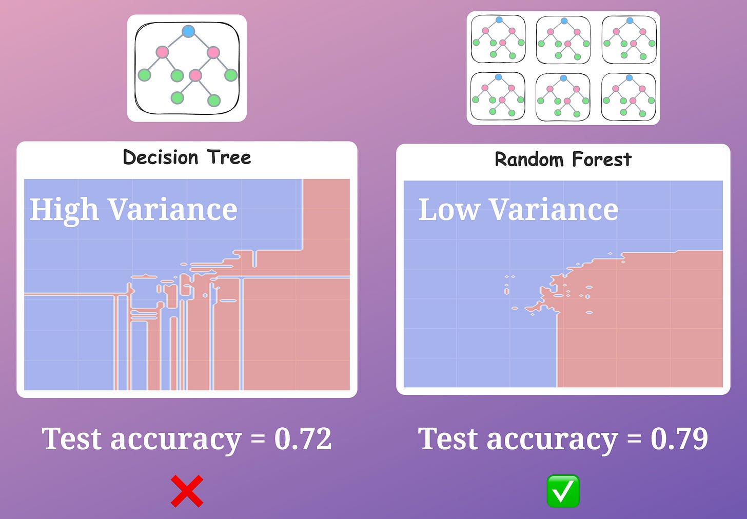
Welcome to the next lesson on tree-based models. In our previous session, you learned how to train and visualize a single decision tree. We saw that while they are highly interpretable, they are also prone to overfitting—capturing noise in the training data and creating overly complex decision boundaries. This sensitivity to the training data is a classic sign of high variance.
Today, we'll address this weakness by exploring Random Forests. This lesson will show you how to train a Random Forest model and, crucially, explain the mechanism it uses—called bagging—to combine many decision trees into a single, more powerful, and less volatile predictor. You'll see how the "wisdom of the crowd" principle applies to machine learning to build more robust models.
1. From a Single Tree to a Forest: The Intuition
A single decision tree can be thought of as a single expert. If that expert has learned from a slightly skewed set of examples, their judgments might be flawed. What if, instead of relying on one expert, we could consult a diverse committee of them and aggregate their opinions? This is the core idea behind a Random Forest.
The algorithm builds an ensemble (a "forest") of decision trees and then gets them to "vote" on a prediction. This process, known as Bootstrap Aggregating or Bagging, is what makes the model so effective.
Let's break down how this is done.
StatQuest: Random Forests Part 1 - Building, Using and Evaluating
The StatQuest video, "Random Forests Part 1," offers a fantastic visual explanation of how a random forest is constructed. Josh Starmer's intuitive style is perfect for understanding these core concepts.
Please watch the following segments to understand the two key randomization techniques: Bootstrap Dataset: See how a new dataset is created by sampling with replacement from the original data. This is the "Bootstrap" part of Bagging. Building Trees: Notice the second layer of randomness—at each split, the tree only considers a random subset of features. Making Predictions: This part explains how the predictions from all the individual trees are combined via majority vote. This is the "Aggregating" part of Bagging.
To summarize the video, a Random Forest introduces two sources of randomness to ensure the trees in the forest are diverse and don't all make the same mistakes:
- Bootstrap Sampling (Bagging): Each tree is trained on a slightly different dataset, created by sampling from the original training data with replacement. This means some data points may be used multiple times in a single tree's training set, while others may be left out entirely.
- Random Feature Subspacing: When deciding on a split, each tree is only allowed to consider a random subset of the available features. This prevents all trees from latching onto the same "super predictive" feature and forces them to explore different data patterns.
The combination of these two techniques creates a forest of de-correlated trees.

2. Why Bagging Reduces Variance
You now have the "how," but the most important question is why this process works. Why does averaging the predictions of many diverse trees lead to a better, more stable model? The answer lies in the relationship between bias and variance.
Understanding the Effect of Bagging on Variance and Bias visually
This article from Towards Data Science provides one of the best visual intuitions for variance reduction.
Please read through the article, focusing on these key ideas: Start at the beginning: The author sets the stage by reminding us that decision trees have low bias but high variance. Bias and Variance of Decision Trees: Look at the first set of plots showing many transparent black decision tree models stacked. Notice how wildly they "wiggle"—this is a visual representation of high variance. An easy Motivation: This section provides a simple statistical analogy. Averaging independent random variables reduces the variance of the result while keeping the mean the same. This is the mathematical principle that underpins bagging. Comparison in one Dimension: The plot comparing the black "tube" (decision trees) to the red "tube" (random forests) is the key takeaway. The random forest predictions are much less spread out, demonstrating a clear reduction in variance. Comparison in two Dimensions: The final heatmaps provide another powerful visualization. The decision tree plots are jagged and vary significantly from one another, while the random forest plots are smooth and consistent.
As the article beautifully illustrates, individual decision trees are high-variance models. A small change in the training data can lead to a completely different tree structure. By training many trees on different subsets of the data and averaging their predictions, we are effectively averaging out their individual errors and "smoothing" the final decision boundary.
- The bias remains roughly the same (if individual trees are unbiased, their average will also be unbiased).
- The variance, however, is significantly reduced because the errors of the individual, de-correlated trees tend to cancel each other out.
This is why a Random Forest is much less likely to overfit than a single decision tree.
3. Training a Random Forest with scikit-learn
Now, let's put this into practice. Training a RandomForestClassifier is very similar to training the DecisionTreeClassifier you used in the last lesson. We'll use the sklearn.ensemble module.
The video below walks through a complete example of training and evaluating a Random Forest model.
Machine Learning Tutorial Python - 11 Random Forest
This video from the codebasics channel provides a clear, hands-on coding session for training a Random Forest.
Watch these two key segments: Training the model: Observe how RandomForestClassifier is imported from sklearn.ensemble and then fitted to the training data. Tuning n_estimators: This part demonstrates the effect of changing the number of trees (n_estimators) in the forest. Notice how the model's score improves as more trees are added, up to a point.
Let's write the code ourselves. We'll use the same Iris dataset from the previous lesson for consistency.
from sklearn.datasets import load_iris
from sklearn.model_selection import train_test_split
from sklearn.ensemble import RandomForestClassifier
from sklearn.metrics import accuracy_score


# Load the iris dataset
iris = load_iris()
X = iris.data
y = iris.target


# Split the dataset
X_train, X_test, y_train, y_test = train_test_split(X, y, test_size=0.3, random_state=42)


# Initialize the Random Forest Classifier
# n_estimators: The number of trees in the forest.
# max_features: The number of features to consider when looking for the best split. 'sqrt' is a common default.
# oob_score=True: Enables a "free" validation score using out-of-bag samples.
rf_classifier = RandomForestClassifier(n_estimators=100,
                                     max_features='sqrt',
                                     oob_score=True,
                                     random_state=42)


# Train the model
rf_classifier.fit(X_train, y_train)


# Make predictions on the test set
y_pred = rf_classifier.predict(X_test)


# Evaluate the model
accuracy = accuracy_score(y_test, y_pred)
print(f"Test set accuracy: {accuracy:.4f}")


# The OOB score is an estimate of accuracy on unseen data
# It is calculated using the samples "left out" of the bootstrap for each tree.
print(f"Out-of-Bag (OOB) score: {rf_classifier.oob_score_:.4f}")
When you run this code, you'll see both the test set accuracy and the Out-of-Bag (OOB) score. The OOB score is a very useful feature of Random Forests. Since each tree is trained on a bootstrap sample, about one-third of the original data is left out. This "out-of-bag" data can be used as a validation set for that specific tree. The OOB score is the average accuracy of each tree on its out-of-bag samples. It's a reliable estimate of the model's performance on unseen data, similar to cross-validation, but without the extra computational cost.
Conclusion
In this lesson, you've made the leap from a single, high-variance decision tree to a robust, low-variance Random Forest. This is a foundational technique in modern machine learning and a powerful tool for your data science toolkit.
Key Takeaways:
- Random Forests are an ensemble method that builds multiple decision trees and aggregates their predictions.
- They reduce variance and prevent overfitting through a process called Bagging (Bootstrap Aggregating).
- Bagging involves two key randomization steps:
- Bootstrap Sampling: Training each tree on a random sample of data drawn with replacement.
- Feature Subspacing: Considering only a random subset of features at each split.
- Averaging the predictions of these diverse, de-correlated trees cancels out individual errors, leading to a more stable and accurate model.
- In
scikit-learn, you can train a Random Forest usingRandomForestClassifierand control its complexity with hyperparameters liken_estimators(number of trees).
In our next lesson, we'll explore another powerful ensemble method: Gradient Boosting. While Random Forests build trees independently and in parallel, Gradient Boosting builds them sequentially, where each new tree is trained to correct the errors made by the previous ones. This offers a different approach to achieving high performance.