CMOS Gate Delays: Propagation and Contamination

1. The Physical Origin of Delay

Why isn't a logic gate's output instantaneous? The answer lies in the physics of the circuit. As an electrical engineering student, you know that any physical wire has resistance and capacitance. In a CMOS circuit, the output of a gate is connected to the inputs of other gates. These connections, along with the transistor gates themselves, create a load capacitance (C_load).

When the input to a gate changes, the pull-up or pull-down network must charge or discharge this C_load. This process isn't instant; it's governed by the RC time constant, where R is the effective resistance of the 'ON' transistors in the network.

• Output going from HIGH to LOW: The pull-down network turns ON, discharging C_load to ground through the nMOS transistors.
• Output going from LOW to HIGH: The pull-up network turns ON, charging C_load from Vdd through the pMOS transistors.

This charging and discharging process is the physical source of delay in CMOS logic.

2. Propagation Delay (t_PD)

Now let's formalize this concept. The propagation delay (t_PD) is an upper bound on the time it takes for a gate's output to become valid and stable after its inputs have become valid. It's the "worst-case" delay; the manufacturer guarantees the gate will have settled to its correct new output value within this time.

Because the charging (pull-up) and discharging (pull-down) paths can have different effective resistances, we distinguish between two types of propagation delay:

• t_PLH: The delay for the output transitioning from Low to High.
• t_PHL: The delay for the output transitioning from High to Low.

The overall propagation delay t_PD for the gate is the maximum of these two: $t_{PD}=\max (t_{PLH},t_{PHL})$.

There are two common ways to measure this delay on a voltage waveform:

1. From 50% to 50%: A common engineering simplification is to measure the delay from the time the input signal crosses 50% of Vdd to the time the output signal crosses 50% of Vdd.
2. Using Logic Thresholds: A more rigorous definition, which connects to our digital abstraction, measures the delay from when the input becomes a valid logic level (crossing V_IH or V_IL) to when the output becomes a valid logic level (crossing V_OH or V_OL).

For a slightly different perspective that uses the 50% measurement point, you can review the lecture slides from UT Austin. They also introduce the common notations t_pdr (rising) and t_pdf (falling).

3. Contamination Delay (t_CD)

While t_PD tells us the longest we have to wait for the output to be correct, contamination delay (t_CD) tells us the shortest amount of time the output is guaranteed to remain at its old, stable value after the inputs start to change. It is a lower bound on the delay.

In other words, after an input transition, you can rely on the old output value for at least t_CD seconds. After that, the output is in an unknown state (it might be changing, or even glitching) until t_PD has passed.

The t_CD specification is crucial for preventing timing errors in sequential circuits, a topic we will cover in detail later in the course. If a data sheet doesn't specify a t_CD, you must make the conservative assumption that t_CD = 0, meaning the output could change instantaneously with the input.

4. Calculating Delays in a Circuit

Now that we understand delays for a single gate, how do we find the total delay of a circuit made of many gates? The principle is straightforward:

• The overall t_PD of a combinational circuit is determined by the longest path from any input to any output. This is called the critical path. You find it by summing the t_PD values of all gates along every possible path and taking the maximum sum.
• The overall t_CD of a circuit is determined by the shortest path from any input to any output. You find it by summing the t_CD values of gates along every path and taking the minimum sum.

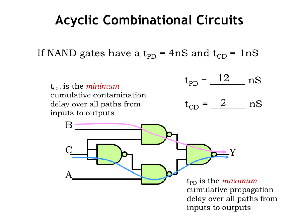
This process is fundamental to timing analysis. Let's read the formal explanation and then watch a video showing a quick method for doing this on a circuit diagram, which is a very useful skill for your exam.

5. A Deeper Look: Estimating Gate Delays

Where do the t_PD numbers for individual gates come from? As we discussed, they are based on the RC time constant. For a simple inverter, this is relatively easy to model. For more complex gates like NAND or NOR, the effective resistance R depends on the number of transistors in series.

For example, in the pull-down network of a 3-input NAND gate, the worst-case (slowest) discharge path is through all three nMOS transistors in series. The resistance of this path is roughly three times that of a single transistor, leading to a longer delay.

A more formal method for estimating the delay in such RC networks is the Elmore delay model. It provides an approximation by summing the resistance-capacitance products for each node in the path. While we won't do detailed Elmore calculations, it's valuable to know that this is a technique used to derive the single t_PD value for a complex gate from its transistor-level structure.

Conclusion

This lesson completes our first module by adding the critical dimension of time to our understanding of CMOS circuits. We've moved from the static behavior of logic gates to their dynamic performance.

Key Takeaways:

• Gate delays are caused by the time it takes to charge and discharge the load capacitance through the resistance of the MOSFETs.
• Propagation Delay (t_PD) is an upper bound on delay. It tells you the maximum time you must wait for a gate's output to be stable and correct after an input change.
• Contamination Delay (t_CD) is a lower bound on delay. It guarantees the minimum time a gate's previous output will remain valid after an input change.
• In a circuit, the overall t_PD is the delay of the longest (critical) path, while the overall t_CD is the delay of the shortest path.

Preview of the Next Lesson

We have now fully covered the fundamentals of the digital abstraction and CMOS technology. In the next module, we will move up a level of abstraction. We will begin our study of Combinational Logic Synthesis and Optimization. The first step will be learning how to formally express any Boolean function using a truth table and derive its canonical sum-of-products (SOP) form, which is a universal way to describe any logic function.