Tracing Kernel Behavior with bpftrace and BCC

1. Getting Started: Installing the Tools

Before we begin, you need to install the necessary tools. The installation process varies slightly by Linux distribution. Since you are building a deep understanding of the kernel, it is highly recommended to work on a modern Linux distribution (like Ubuntu 20.04+, Fedora 33+, or Debian 11+) either on a bare-metal machine or in a VM. These newer versions have better out-of-the-box support for eBPF.

The following resource provides installation instructions for both bpftrace and bcc.

2. bpftrace: The Swiss Army Knife for Ad-Hoc Tracing

bpftrace is a high-level tracing language that allows you to write powerful tracing scripts, often as a single line of code (a "one-liner"). It uses a syntax inspired by awk and DTrace, making it incredibly expressive for on-the-fly system exploration.

The basic structure of a bpftrace program is:

probe_specifier /filter/ { action }

• Probe Specifier: Defines where to instrument (e.g., a kernel function, a tracepoint).
• Filter: An optional condition to decide when to run the action.
• Action: The code to execute what to do when the probe fires and the filter passes.

Let's walk through building your first bpftrace commands.

Key bpftrace One-Liner Patterns

The video gave you a solid foundation. Now let's explore some of the most common and powerful patterns you'll use for performance analysis, which directly leverage the in-kernel aggregation capabilities we discussed in the last lesson.

The following one-liners are from Brendan Gregg's excellent bpftrace tutorial. Try running them on your system to see them in action.

• Counting Events by Group:
  This is one of the most fundamental patterns. Let's count how many system calls each process is making.

  
  
  
  # Count syscalls by process name. Press Ctrl-C to see the summary.
  sudo bpftrace -e 'tracepoint:raw_syscalls:sys_enter { @[comm] = count(); }'
  

  Here, @[comm] = count(); is the core. @[] defines a map. We are creating a map where the key is the process name (comm) and the value is an automatically incrementing counter. All this counting happens efficiently inside the kernel.

• Creating a Latency Histogram:
  Let's measure the size of data returned by read() system calls and display it as a histogram.

  
  
  
  # Show a distribution of read() return sizes for a specific PID (replace 1234 with a PID on your system).
  # You can find PIDs using 'ps aux'.
  sudo bpftrace -e 'tracepoint:syscalls:sys_exit_read /pid == 1234/ { @bytes = hist(args->ret); }'
  

  The hist() function collects the values (in this case, the return value args->ret from the read syscall) and automatically generates a power-of-2 logarithmic histogram. This is perfect for understanding the distribution of latencies or sizes.

• Timing Function Execution:
  This is the practical implementation of the interview scenario from our previous lesson. We use two probes: one at the function entry (kprobe) to record a start time, and one at the function return (kretprobe) to calculate the duration.

  
  
  
  # Time the duration of vfs_read() calls and show a histogram by process name.
  sudo bpftrace -e 'kprobe:vfs_read { @start[tid] = nsecs; } kretprobe:vfs_read /@start[tid]/ { @ns[comm] = hist(nsecs - @start[tid]); delete(@start[tid]); }'
  

  Let's break this down:

  1. kprobe:vfs_read { @start[tid] = nsecs; }: When entering vfs_read, we store the current timestamp (nsecs) in a map named @start, keyed by the thread ID (tid).
  2. kretprobe:vfs_read /@start[tid]/: When returning from vfs_read, we first use a filter (/@start[tid]/) to ensure we only proceed if we have a saved start time for this thread.
  3. { @ns[comm] = hist(nsecs - @start[tid]); delete(@start[tid]); }: We calculate the latency, add it to a histogram map named @ns (keyed by process name), and then delete the entry from our @start map to clean up.

These patterns—counting, histograms, and timing—are the building blocks for countless performance investigations. For more complex logic, you can save your bpftrace code into a file (e.g., myscript.bt) and run it with sudo bpftrace myscript.bt.

3. BCC Tools: A Curated Toolbox for Common Problems

While bpftrace is excellent for custom queries, you often don't need to write a script from scratch. The BCC (BPF Compiler Collection) provides a rich set of powerful, ready-to-use tools for common performance analysis tasks. These are typically Python scripts that have the eBPF C code embedded within them.

For your goal of cracking interviews and becoming a proficient kernel developer, knowing which BCC tool to reach for is a critical skill.

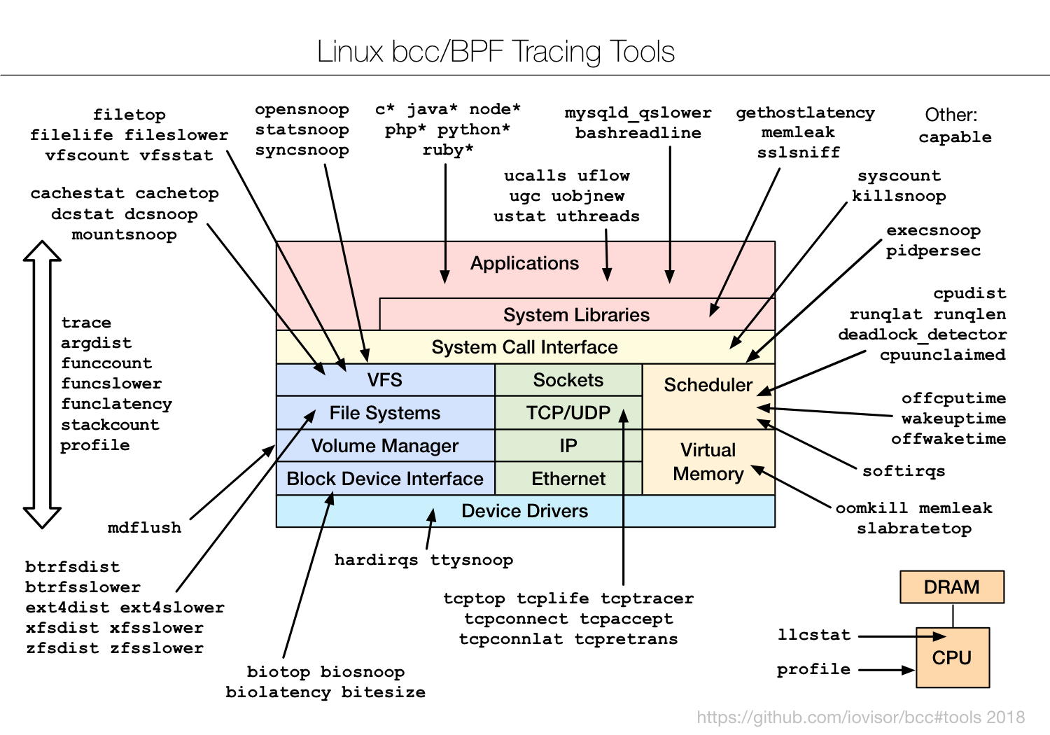
Let's see some of these tools in action.

Quick Reference for Essential BCC Tools

Here is a summary of the tools demonstrated, along with a few others you should be aware of. Most are installed in /usr/share/bcc/tools.

This is just a small sample. Exploring the /usr/share/bcc/tools directory on your system is a great way to discover the full range of available tools.

4. Interview Scenario: Diagnosing Application Sluggishness

Interviewer: "A database server is reporting periodic slowdowns. Users complain that some queries take much longer than expected. We suspect I/O issues, but iostat shows that the average disk utilization isn't abnormally high. How would you use eBPF-based tools to pinpoint the root cause?"

Conclusion

In this lesson, you have moved from the theory of eBPF to its practical application. You've learned how to wield both bpftrace and the BCC tool collection to gain deep visibility into kernel and application behavior.

Key Takeaways:

• bpftrace is a high-level language for writing custom, ad-hoc tracing one-liners and scripts. It's your tool for exploration and asking novel questions of the system.
• BCC is a collection of pre-built, expert-written tools that solve common performance problems. They are your first stop for diagnosing issues related to processes, files, disk I/O, networking, and more.
• The fundamental patterns of counting, creating histograms, and timing events are the building blocks of performance analysis with eBPF.
• A methodical diagnostic approach—starting broad and narrowing down—is key to efficiently solving complex performance problems with these tools.

Preview of the Next Lesson:

Now that you're equipped with a powerful set of tracing tools, we'll focus on a specific and notoriously difficult performance challenge: lock contention. In the next lesson, you will learn to use profiling tools to identify a lock contention bottleneck and apply an appropriate resolution strategy. We'll see how the tracing skills you've developed today are essential for understanding and resolving these concurrency issues.