Cost Variance Decomposition

1. The Foundation: Standard Costing

Before we can analyze variances, we need to understand what we are comparing against. In most manufacturing and production environments, this "what-if" scenario is the standard cost.

A standard cost is a carefully predetermined cost for producing a single unit of output. It's built from two key elements:

• Standard Price (or Rate): The expected price for one unit of input (e.g., $20 per labor hour, $1.50 per kWh of electricity).
• Standard Quantity: The expected amount of input needed to produce one unit of output (e.g., 6 labor hours per product).

Variance analysis is the process of comparing the actual costs incurred against the standard cost for the actual level of production.

2. Decomposing Variable Cost Variances

Variable costs, such as direct labor and variable manufacturing overhead (e.g., electricity for machines), change in proportion to production volume. We can break down the total variance for these costs into two primary components: a rate (or price/spending) variance and an efficiency (or usage/quantity) variance.

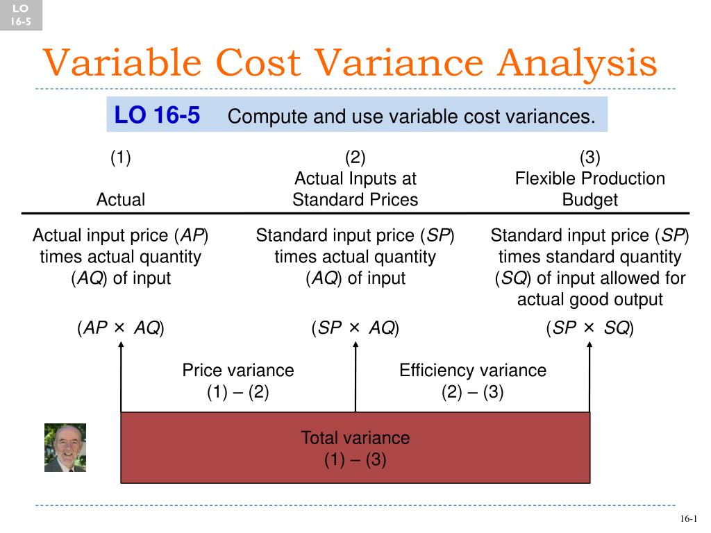
The logic is to isolate one effect at a time:

• Rate/Spending Variance: Did we pay more or less than the standard rate for the inputs we used?
• Efficiency/Usage Variance: Did we use more or less input than the standard allowance for the output we produced?

Let's see how this applies to Direct Labor and Variable Overhead.

2.1. Direct Labor Variance

Direct labor is a classic variable cost. Its total variance is decomposed as follows:

1. Labor Rate Variance: This measures the difference between the standard rate and the actual rate paid to employees, multiplied by the actual hours worked. A common cause for this variance is using higher-paid employees for tasks planned for junior staff, or unexpected overtime payments.

   $$\text{Labor Rate Variance}=(\text{Standard Rate}-\text{Actual Rate})\times \text{Actual Hours}$$

2. Labor Efficiency Variance: This measures the difference between the standard hours that should have been worked for the actual output and the actual hours that were worked. It is a key indicator of worker productivity or operational efficiency.

   $$\text{Labor Efficiency Variance}=(\text{Standard Hours for Actual Output}-\text{Actual Hours})\times \text{Standard Rate}$$

Notice we use the Standard Rate here to isolate the pure effect of using more or fewer hours, without confounding it with the rate variance.

2.2. Variable Overhead Variance

The analysis for variable overhead is very similar to direct labor, especially when overhead costs are allocated based on labor hours.

1. Variable Overhead Spending Variance: This is analogous to the Labor Rate Variance. It measures the difference between what you expected to spend per activity unit (e.g., per labor hour) and what you actually spent.

   $$\text{VOH Spending Variance}=(\text{Standard Rate}-\text{Actual Rate})\times \text{Actual Hours}$$

2. Variable Overhead Efficiency Variance: This is analogous to the Labor Efficiency Variance. It measures the cost impact of taking more or less time (hours) than the standard allows for the actual production output.

   $$\text{VOH Efficiency Variance}=(\text{Standard Hours for Actual Output}-\text{Actual Hours})\times \text{Standard Rate}$$

To see these calculations in action, we'll return to the Commerce Specialist video. It provides a clear, worked-out example.

3. Decomposing Fixed Cost Variances

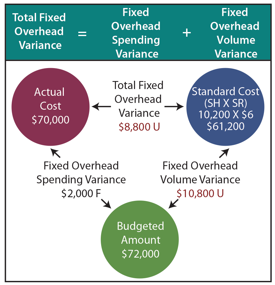
Fixed costs, like factory rent or salaried manager pay, do not change with production volume (within a relevant range). Therefore, their analysis is different. We don't have a true "efficiency" variance in the same way. Instead, we split the total variance into a spending component and a volume component.

1. Fixed Overhead Spending (or Budget) Variance: This is the simplest variance. It's the difference between the budgeted fixed overhead and the actual fixed overhead incurred.

   $$\text{FOH Spending Variance}=\text{Budgeted FOH}-\text{Actual FOH}$$

2. Fixed Overhead Volume Variance: This variance is more conceptual. It arises because, for accounting purposes, we "absorb" or "apply" fixed overhead to products at a predetermined rate (e.g., $10 of fixed OH per unit). The volume variance measures the impact of producing more or fewer units than the budgeted volume used to set that rate.

   • If you produce more than budgeted, you over-absorb your fixed costs, resulting in a favorable volume variance.
   • If you produce less than budgeted, you under-absorb your fixed costs, resulting in an unfavorable volume variance. This signals underutilization of capacity.
   $$\text{FOH Volume Variance}=\text{Absorbed FOH}-\text{Budgeted FOH}$$

   Where Absorbed FOH = Standard Rate per Unit * Actual Units Produced.

3.1. Advanced Decomposition: Fixed Overhead Efficiency and Capacity

For a deeper analysis, particularly valued in senior FP&A roles, the Volume Variance can be broken down further into Efficiency and Capacity variances. This is crucial for understanding why volume differed from the plan.

• FOH Efficiency Variance: This is identical in calculation to the labor efficiency variance. It asks: for the units we produced, did our team work efficiently? It isolates the productivity of the workforce.

  $$\text{FOH Efficiency Variance}=(\text{Std. Hours for Actual Output}-\text{Actual Hours})\times \text{Std. FOH Rate per Hour}$$

• FOH Capacity Variance: This variance compares the hours you actually worked to the hours you budgeted to work. It measures how well you utilized your potential production time.

  $$\text{FOH Capacity Variance}=(\text{Actual Hours}-\text{Budgeted Hours})\times \text{Std. FOH Rate per Hour}$$

The following video provides an excellent, comprehensive walk-through of the entire fixed overhead variance decomposition, including these more advanced components.

4. Consolidated View and Reference

To help you organize these concepts, a formal accounting text can provide a structured summary of all the formulas. This aligns with your goal of having access to high-quality reference materials.

Conclusion

Congratulations! You have now built a comprehensive framework for analyzing the key drivers of cost performance. By moving beyond a simple "actual vs. budget" comparison, you can provide management with actionable insights into pricing, productivity, and capacity utilization.

Key Takeaways:

• Variable Costs (like labor) are decomposed into a Rate Variance (did we pay the right price?) and an Efficiency Variance (did we use the right quantity?).
• Fixed Costs are decomposed into a Spending Variance (did we stick to the budget?) and a Volume Variance (did our production level absorb the budgeted fixed costs?).
• The Fixed Overhead Volume Variance can be further broken down into an Efficiency Variance (how productively did we work?) and a Capacity Variance (how much of our available time did we use?).
• This detailed decomposition allows you to ask targeted questions to operational managers and become a true strategic partner to the business.

In our next lesson, we will focus on communicating these findings. You will learn to perform bridge (waterfall) analysis to visually explain period-over-period changes in key financial metrics. This will allow you to take the variances you've just calculated and present them in a clear, compelling narrative for executive leadership.