Revolving Credit & Debt Schedules: Amortization & Interest

1. Introduction to Debt Schedules

A debt schedule is a table within a financial model that tracks a company's debt obligations over time. Its primary purpose is to forecast the ending debt balance, principal repayments, and interest expense for each period.

To get a clear overview of the different types of debt schedules and their purpose, we'll start with a foundational video.

As the video explained, the core logic is driven by a company's cash position relative to a minimum cash balance it needs to operate.

• Cash Surplus: Excess cash can be used to repay debt.
• Cash Deficit: The company must borrow money to cover the shortfall.

For our three-statement model, we will model two primary types of debt:

1. Long-Term Debt: This represents debt with a maturity of more than one year, often with a scheduled repayment of the principal over time. This scheduled repayment is called principal amortization.
2. Revolving Credit Facility (or "Revolver"): This is like a corporate credit card. It's a flexible credit line that a company can draw on to cover short-term cash shortfalls and repay as soon as it has surplus cash. It's the first line of defense against a liquidity crunch.

The structure of a debt schedule for long-term debt is a "roll-forward" calculation, very similar to the PPE schedule we built earlier.

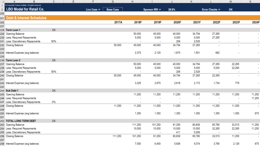
This roll-forward logic is key:

2. The Engine: Cash Flow for Debt Repayment

Before we can model any repayments or borrowings, we must first calculate the amount of cash the company generates to service its debt. This is the central driver of the entire debt schedule. We'll call this the Cash Flow Surplus / (Deficit).

The formula is conceptually simple:

Let's refine this. "Cash Generated" is essentially the company's free cash flow before any financing activities. "Minimum Cash Required" is a policy decision—a safety buffer the company wants to maintain.

The detailed calculation looks like this:

1. Start with Cash at the Beginning of the Period.
2. Add all cash inflows and outflows from operations and investing. (This is often simplified to Cash Flow from Operations - CapEx).
3. Subtract any Mandatory Debt Repayments. We must make these payments, so the cash is not available for anything else.
4. Subtract the Minimum Cash Balance the company must hold for operational needs.

The result tells us if we have a surplus to repay debt or a deficit that requires borrowing.

This is a critical calculation. Let's see it in action.

The accompanying article, "Debt Schedule: Video Tutorial and Excel Example" from Breaking Into Wall Street (LINK), provides a static image of this calculation under Step 2 of the LBO section, which can be a helpful reference.

3. Modeling the Revolving Credit Facility

The revolver is the first tool used to manage the cash surplus or deficit. Its logic is straightforward:

• If we have a cash deficit, we draw down on the revolver to bring our cash balance back up to the minimum.
• If we have a cash surplus, we first use it to repay any outstanding balance on the revolver before using it for anything else.

A common and efficient way to model this in Excel is by using the MIN and MAX functions.

Key Logic using MIN/MAX:

• Revolver Drawdown (Addition): =MAX(0, -Cash_Surplus_Deficit)
  • This formula returns the deficit amount as a positive number (a drawdown) and 0 if there's a surplus.
• Revolver Repayment (Paydown): =-MIN(Beginning_Revolver_Balance, Cash_Surplus_Deficit)
  • This formula calculates the repayment amount, ensuring it's never more than the outstanding revolver balance or the available cash surplus. It's negative because it's a cash outflow.

4. Modeling Long-Term Debt Repayments

After accounting for any revolver activity, we can address the long-term debt. Repayments fall into two categories:

1. Mandatory Amortization: This is the scheduled principal repayment specified in the loan agreement. It's a non-negotiable payment. You can read more about it in the Wall Street Prep article "Debt Schedule" (LINK) in "Step 3. Mandatory Loan Repayment Percentage Assumptions".
2. Optional Repayments (Cash Sweep): If there is still a cash surplus after making mandatory payments and handling the revolver, the company may choose to repay long-term debt ahead of schedule. A "cash sweep" is a common feature where a certain percentage (e.g., 50%) of this excess cash is automatically used to pay down debt.

The order of operations is critical and is often called a "cash flow waterfall":

1. Calculate Cash Flow Surplus / (Deficit).
2. Draw on / repay the revolver.
3. Pay mandatory amortization on long-term debt.
4. Use any remaining cash for optional repayments (cash sweep).

5. Calculating Interest Expense and the Circularity Problem

The final piece is calculating interest expense for the income statement.

The formula is: Interest Rate × Debt Balance. However, since the debt balance changes during the period, we should use the average debt balance.

This applies to each tranche of debt, including the revolver.

This calculation introduces a famous problem in financial modeling: a circular reference.

Think it through:

1. Interest Expense depends on the Average Debt Balance.
2. The Ending Debt Balance (which is part of the average) depends on repayments.
3. Repayments depend on the Cash Flow Surplus.
4. Cash Flow Surplus depends on Net Income.
5. Net Income depends on Interest Expense!

We have a loop: Interest Expense → Ending Debt → Net Income → Interest Expense.

Excel will flash a warning about this. For today, you just need to recognize this problem exists. In a professional setting, there are several ways to solve it, such as enabling iterative calculations in Excel or using a "toggle switch" (often called a circuit breaker). We will dedicate a future lesson (4.8 Resolve circular references...) to resolving this properly. For now, a common simplification is to calculate interest based on the beginning-of-period debt balance to avoid the circularity.

Conclusion

Excellent work. We've constructed the logic for one of the most intricate and important supporting schedules in a financial model. You've learned how a company's cash flow dictates its ability to manage its debt, and how to model the mechanics of both flexible revolvers and structured long-term debt.

Key Takeaways:

• A debt schedule is a roll-forward that tracks debt balances, repayments, and interest.
• The schedule is driven by the Cash Flow Surplus / (Deficit), which determines if the company needs to borrow or can repay debt.
• The revolver acts as a short-term liquidity plug, managed first in the "cash flow waterfall."
• Long-term debt is paid down via mandatory amortization and optional repayments (cash sweeps).
• Calculating interest on average balances creates a circular reference, a classic modeling challenge that we will solve in a later lesson.

In our next lesson, we will begin the final assembly of our model. We will take the outputs from our supporting schedules (Working Capital, CapEx, Headcount, and now Debt) and link the income statement and balance sheet via retained earnings and other equity accounts. This is where everything starts to come together.