Regression-Based Forecasting: Integration and Validation

1. From Equation to Dynamic Forecast Model

After running and validating your regression analysis, you are left with a powerful equation. For a simple linear regression, it looks like this:

$\text{Forecasted Value}=\text{Intercept}+(\text{Coefficient}\times \text{Future Driver Value})$

For a multiple regression with two drivers, it expands to:

$\text{Forecasted Value}=\text{Intercept}+(C_1\times D_1)+(C_2\times D_2)$

Our goal is to build this equation into Excel in a way that is robust and easy to update. The key principle is to never hard-code the coefficients into your formulas. Instead, you should always link to the cells in the regression SUMMARY OUTPUT sheet. This ensures that if you re-run the regression with new data, your forecast model updates automatically.

Let's look at a practical example. Imagine we've found a significant relationship between advertising expenses and revenue.

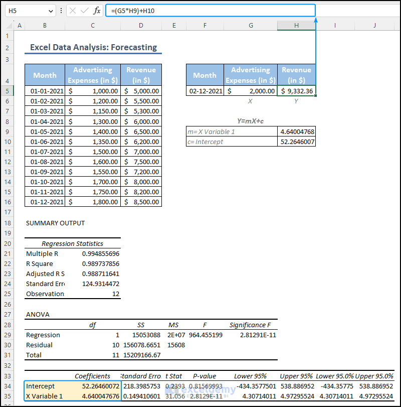
The formula to forecast revenue for a new Advertising Expenses value of $1,600 (cell C10) would be:

=C16 + C17*C10

Where:

• C16 is the cell containing the Intercept coefficient (-235.15).
• C17 is the cell containing the Advertising Expenses coefficient (2.63).
• C10 is the cell containing our assumption for the future driver value.

This same logic applies seamlessly to multiple regression.

The formula shown, =G2+F2*A15+E2*B15, is a direct translation of the multiple regression equation, using cell references for the intercept (G2), the first coefficient (F2), the second coefficient (E2), and the new driver values (A15 and B15).

More Dynamic Methods in Excel

While linking to the output sheet is excellent practice, Excel offers functions that can make this process even more dynamic. The following resource discusses several options for using regression results.

• Option #3 (INDEX and LINEST) is particularly powerful for advanced modelers. It allows you to extract the coefficients directly into cells with a formula, meaning you don't even need to re-run the Data Analysis ToolPak manually to update your model.
• Option #4 (FORECAST.LINEAR) is a quick and easy function, but be aware that it only works for simple (one-variable) linear regression.

For most financial models, the cell-referencing method we first discussed offers the best balance of transparency, control, and dynamism.

2. Validating Accuracy: Beyond a Single Number

A single-point forecast, like "$1,500,000 in sales," is precise but misleading. Every forecast has inherent uncertainty. A top-tier analyst communicates this uncertainty. Just as in civil engineering, where you design with tolerances and safety factors, in financial modeling, we must present our forecasts with a quantified margin of error.

The Standard Error of the Regression

First, let's revisit the Standard Error of the Regression from your SUMMARY OUTPUT. This value represents the typical distance between the historical data points and the regression line. It serves as a fundamental measure of your model's predictive accuracy.

If your model forecasts sales of $500k and the standard error is $25k, you can give a rough "rule of thumb" estimate that the actual result is likely to fall within the range of $475k to $525k.

The following reading explains this concept.

Constructing Confidence Intervals

The most professional way to present a forecast is with a confidence interval. This provides a range within which you expect the true value to fall, with a certain level of confidence (typically 90% or 95%).

A 95% confidence interval of [$475k, $525k] means you are 95% confident that the actual sales figure will fall within this range.

The formula to approximate a confidence interval around your point forecast (Ŷ) is:

$\text{Confidence Interval}=\hat{Y}\pm (t_{\alpha /2,n-k-1}\times \text{SE})$

Where:

• $\hat{Y}$ is your point forecast from the regression equation.
• $\text{SE}$ is the Standard Error of the Regression from your output.
• $t$ is the "t-value" from the t-distribution. This value depends on your desired confidence level (e.g., 95%) and your model's "degrees of freedom" (found in the ANOVA table as Residual df).

You don't need to look up t-values in a statistical table. Excel's T.INV.2T function does it for you. The syntax is T.INV.2T(probability, degrees_freedom), where probability is 1 - confidence_level (e.g., 0.05 for 95% confidence).

Let's see how this is done in practice.

Best Practice: Out-of-Sample Validation

The truest test of a forecast model's predictive power is to test it on data it has never seen before. A common best practice is to:

1. Hold out a portion of your historical data (e.g., the last 4 quarters).
2. Build your regression model using only the earlier data (the "training" set).
3. Use the resulting equation to "forecast" the results for the 4 quarters you held out.
4. Compare your forecasts to the actuals for those 4 quarters.

This "out-of-sample" testing gives you a much more realistic measure of how your model will perform in the future than simply looking at the $R^2$ on the data it was built on.

Conclusion

You have now completed the regression forecasting process, from identifying drivers to building and validating a dynamic model. This journey from raw data to a statistically sound forecast with quantified uncertainty is a cornerstone of advanced financial analysis.

Key Takeaways:

• Integrate Dynamically: Always build forecast formulas by linking to the cells in your regression output, not by hard-coding numbers.
• Quantify Uncertainty: Use the Standard Error as a quick measure of accuracy, but use Confidence Intervals for professional-grade reporting.
• Present a Range: A single-point forecast is rarely enough. Communicating a forecast range manages expectations and demonstrates analytical rigor.
• Test on New Data: The best models prove their worth on data they haven't seen before. Keep the concept of out-of-sample testing in mind for important forecasts.

This lesson concludes our module on Financial Forecasting Techniques. We've covered time series methods, correlation, and a deep dive into regression analysis.

In our next module, we will change gears and begin constructing a full Three-Statement Financial Model. You'll apply your forecasting skills as we build the detailed supporting schedules for working capital, capital expenditures, and debt that form the engine of a comprehensive financial model.