Introduction
In our previous lesson, we explored how to maximize the value of existing resources by analyzing and improving fleet-wide efficiency. We saw how Google uses systems like GWP and Borg to measure resource consumption and reclaim waste, turning potential slack into massive cost savings. Now that we understand how to get the most out of the hardware we have, we'll address the forward-looking challenge: ensuring we have the right amount of hardware for the future.
This lesson will guide you through how to formulate a capacity plan for a distributed system considering growth forecasts and SLOs. This is a core strategic responsibility for a Principal Engineer. It's a multidisciplinary exercise that sits at the intersection of systems engineering, statistics, and business planning. A successful capacity plan ensures your service remains reliable and performant as it grows, without incurring wasteful over-provisioning. We will start with the fundamental principles and then explore the sophisticated, automated systems that companies like Google and Netflix use to manage this complexity at scale.
Resource Provisioning vs. Capacity Planning
To begin, it's crucial to distinguish between two related but distinct activities: resource provisioning and capacity planning. The Google SRE article "Best Practices for Capacity Management" provides a clear definition.
SRESRE Best Practices for Capacity Management
This article from Google SREs clearly separates the tactical problem of provisioning from the strategic one of planning.
Please read the introduction to understand the core principles (first few paragraphs), the section on complexities (pages 50), and the conclusion (first paragraph). Focus on the distinction between the two key questions the article poses.
As the article explains, the two concepts answer different questions:
- Resource Provisioning (Tactical): "How do I keep the service running right now?" This involves allocating the correct resources for the current demand, considering peak usage and immediate reliability needs.
- Capacity Planning (Strategic): "How do I keep the service running for the foreseeable future?" This involves forecasting future demand and ensuring the supply of resources will be available to meet it.
Your role as a Principal Engineer primarily involves the strategic side—capacity planning. However, a sound strategic plan must be built upon a solid tactical foundation. Let's examine the components of that foundation.
The Building Blocks of a Capacity Plan
A capacity plan translates business goals into a concrete resource acquisition strategy. The three primary inputs are the service's SLOs, the demand forecast, and the performance model of the system itself.
1. Service Level Objectives (SLOs) and Redundancy
Your service's availability SLO is a primary driver of capacity. A high-availability target requires building in redundancy to tolerate failures, and that redundancy has a direct cost in terms of capacity.
This is typically expressed as N+x redundancy, where 'N' is the number of components (e.g., tasks, regions) needed to serve the load, and 'x' is the number of spare components that can fail without impacting the service.
Complexities of Capacity Management for Distributed Services
This Google TechTalk on capacity management provides a detailed walkthrough of how redundancy impacts resource provisioning.
Please watch the segment from redundancy concepts. The speaker explains task-level and region-level redundancy (N+1, N+2) and, crucially, walks through a calculation showing how running in more regions can make N+2 redundancy significantly more cost-effective.
As the video and the SRE paper explain, provisioning for N+2 in a 3-region setup means each region must be able to handle 100% of the global load (since two regions could fail). This results in a maximum "level-flight" utilization of only 33%, which is quite inefficient. However, in a 5-region setup, the remaining three regions only need to absorb the load, so each replica is smaller. This raises the level-flight utilization to nearly 60%, almost halving the overhead cost of N+2 redundancy.
This calculation demonstrates a critical trade-off: higher availability SLOs demand more redundancy, which directly increases the required capacity and cost.
2. Demand Forecasting and Target Utilization
The second input is the demand forecast. This includes:
- Organic Growth: The natural increase in usage from the existing user base.
- Inorganic Growth: Spikes in demand from new feature launches, marketing campaigns, or expansion into new markets.
You cannot simply provision capacity to match the average expected demand. As we've discussed, systems do not behave linearly as they approach their physical limits.
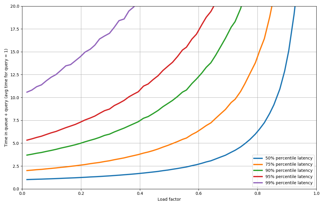
This non-linear relationship is why we must operate at a specific target utilization well below 100%. A capacity plan doesn't aim to keep average utilization at, say, 95%. It aims to ensure that even at peak demand, utilization stays below a safe target that honors the latency SLO.
The Google TechTalk provides an excellent summary of the factors that contribute to this "headroom."
Complexities of Capacity Management for Distributed Services
Here, the speaker breaks down all the reasons why the ideal target utilization is much lower than 100%.
Watch the summary of these factors from target utilization summary. He recaps how the need to avoid non-linear performance degradation, accommodate redundancy, handle latency-insensitive batch loads, and leave a buffer for unknown events all combine to lower the effective target utilization.
A robust capacity plan models the expected peak demand (including growth) and calculates the total resources needed so that this peak load results in a utilization no higher than the designated target.
3. System Performance Model
The final piece is the performance model: how much of each resource (CPU, memory, network IO) does a single unit of demand (e.g., a request) consume? This is what connects the demand forecast to a concrete resource number.
For a simple service, this might be a back-of-the-envelope calculation. For complex systems at Google scale, this is a far more involved process. A paper on capacity analysis offers a glimpse into the formal, mathematical approach.
[PDF] Capacity Analysis of Distributed Computing Systems with Multiple ...
This paper provides a formal definition of system capacity that is highly relevant to your background in computer science.
Skim the introduction and system model. The key takeaway is Definition 1, where the authors define ε-capacity (the definition). This is the formal expression of an SLO: the maximum number of tasks (M) the system can support such that the probability of overload is no more than ε. Then look at Theorem 1 and Theorem 2 (Theorems 1 and 2) which provide analytical bounds on this capacity.
This theoretical framing shows that capacity planning can be modeled rigorously. The ε in ε-capacity is, in essence, your error budget. While most practical planning doesn't involve solving these exact equations, the underlying principles are the same: we are trying to find the maximum sustainable load for a given reliability target.
From Theory to Practice: Automated Capacity Planning
Manually calculating capacity across hundreds of services, each with multiple resource dimensions, regions, and uncertain growth forecasts, is intractable. At Google and other large tech companies, this process is highly automated.
Let's look at the system Netflix developed, as it provides an excellent, well-documented public example of these principles in action.
AWS re:Invent 2022 - Capacity plan optimally in the cloud (NFX304)
This AWS re:Invent talk by an engineer from Netflix details their automated capacity planning system. It's a masterclass in applying modeling and simulation to a complex business and engineering problem.
Watch the following key segments to understand their approach: Modeling Uncertainty: First, see how they capture user forecasts not as single numbers but as probability distributions to model uncertainty. Watch the segments on user input as intervals and how the final user desire is a composition of user input and default workload characteristics. The "Least Regret" Framework: Next, understand how they use Monte Carlo simulation to find the "least regretful" cluster. Watch from Monte Carlo simulation to understand the concept of a regret function that prices the cost of under-provisioning vs. over-provisioning. Worked Example: Finally, see a concrete example of this in action, from a large-interval example. Notice how even with a highly uncertain input (100k to 1M writes/sec), the process yields a specific, defensible cluster choice.
This approach is incredibly powerful. Key takeaways from the Netflix model include:
- Embrace Uncertainty: User forecasts are rarely perfect. By modeling them as intervals or distributions (e.g., a Beta distribution), the plan can account for this uncertainty.
- Compose Inputs: The final "desire" is a combination of what the user provides (e.g., estimated QPS, data size) and what the workload owner provides (e.g., compression ratio, CPU cost per operation).
- Optimize for "Least Regret": Using Monte Carlo simulation, the system evaluates thousands of possible future scenarios against many potential hardware configurations. It then selects the configuration that minimizes "regret"—a cost function that balances the risk of outages (under-provisioning) against the risk of wasted money (over-provisioning).
- Parameterize Business Logic: The regret function is tunable. A startup might weight over-provisioning cost very highly, while a mature, critical service at Google would weight under-provisioning (outage risk) much higher.
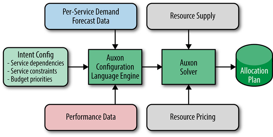
This automated, probabilistic approach is state-of-the-art. Google's internal systems for capacity planning, such as Auxon, operate on similar principles.
Closing the Loop: Monitoring the Plan
A capacity plan is a hypothesis. Once deployed, you must monitor its performance to validate your assumptions and feed corrections back into the model. The Netflix talk concludes with an essential point about what to monitor.
AWS re:Invent 2022 - Capacity plan optimally in the cloud (NFX304)
This final segment covers how to monitor the effectiveness of your plan in production.
Watch the section from monitoring your choices. The key insight is to monitor metrics that are direct proxies for saturation, not just raw utilization. For CPU, this means worker queuing delay, not just CPU usage.
If your CPU worker threads are never queued, buying more CPUs won't make your application faster, even if utilization is high. Conversely, if queuing is high, you are CPU-bound and need more capacity. For other resources like memory, proxy metrics like page cache hit rate or disk flush frequency can be better indicators of pressure than raw memory usage. This monitoring data is the feedback loop that makes the entire planning process adaptive and accurate over time.
Conclusion
In this lesson, we've constructed a comprehensive framework for capacity planning. You've seen how it extends beyond simple trend-line extrapolation into a sophisticated modeling exercise that balances reliability, performance, and cost.
Your key takeaways are:
- Plan vs. Provision: Capacity planning is the strategic, long-term forecasting of resource needs, while provisioning is the tactical, immediate allocation of those resources.
- SLOs Drive Capacity: Availability SLOs determine the required redundancy (
N+x), which is a primary cost driver. Latency SLOs determine the maximum safe target utilization. - Model the System: A robust plan requires a model that translates demand (QPS, users) into resource consumption (CPU, RAM, disk, network).
- Automate with Uncertainty: Modern capacity planning at scale is automated. It embraces the uncertainty of forecasts by using probability distributions and simulation (e.g., Monte Carlo) to find an optimal, "least regretful" solution.
- Monitor for Saturation: To validate your plan, monitor metrics that indicate saturation (like queuing delay), not just raw utilization. This provides the crucial feedback loop for refining your models.
In our next lesson, we will delve deeper into the economic side of this equation. Having planned for the right amount of capacity, we will explore how to devise cost-optimization strategies for a large-scale cloud-native system while maintaining performance SLOs. This will involve looking at instance selection, reserved instances, autoscaling, and other levers to ensure your well-planned system is also maximally cost-effective.